
A to Z of Excel Functions: The LINEST Function
4 October 2021
Welcome back to our regular A to Z of Excel Functions blog. Today we look at the LINEST function.
The LINEST Function

Sometimes, you wish to forecast what comes next in a sequence, i.e. make a forecast. There are various approaches you could use:
- Naïve method: this really does live up to its billing – you simply use the last number in the sequence, e.g. the continuation of the series 8, 17, 13, 15, 19, 14, … would be 14, 14, 14, 14, … Hmm, great
- Simple average: only a slightly better idea: here, you use the average of the historical series, e.g. for the continuation of the series 8, 17, 13, 15, 19, 14, … would be 14.3, 14.3, 14.3, 14.3, …
- Moving average: now we start to look at smoothing out the trends by taking the average of the last n items. For example, if n were 3, then the sequence continuation of 8, 17, 13, 15, 19, 14, … would be 16, 16.3, 15.4, 15.9, 15.9, …
- Weighted moving average: the criticism of the moving average is that older periods carry as much weighting as more recent periods, which is often not the case. Therefore, a weighted moving average is a moving average where within the sliding window values are given different weights, typically so that more recent points matter more. For example, instead of selecting a window size, it requires a list of weights (which should add up to 1). As an illustration, if we picked four periods and [0.1, 0.2, 0.3, 0.4] as weights, we would be giving 10%, 20%, 30% and 40% to the last 4 points respectively which would add up to 1 (which is what it would need to do to compute the average). Therefore the continuation of the series 8, 17, 13, 15, 19, 14, … would be 15.6, 15.7, 15.7, 15.5, 15.6, …
All of these approaches are simplistic and have obvious flaws. We are using historical data to attempt to predict the next point. If we go beyond this, we are then using forecast data to predict further forecast data. That doesn’t sound right. We should stick to the next point. Since we are looking at a single point and we can weight the historical data by adding exponents to the calculation, this is sometimes referred to as Exponential Single Smoothing.
A slightly more sophisticated method is called regression analysis: well, that takes me back! This is a technique where you plot an independent variable on the x (horizontal axis) against a dependent variable on the y (vertical) axis. “Independent” means a variable you may select (e.g. “June”, “Product A”) and dependent means the result of that choice or selection.
For example, if you plotted your observable data on a chart, it might look something like this:
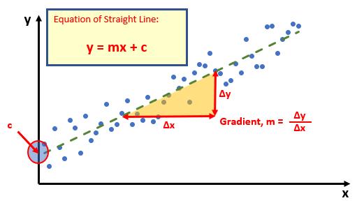
Do you see? You can draw a straight line through the data points. There is a statistical technique where you may actually draw the “best straight line” through the data using an approach such as Ordinary Least Squares, but rather than attempt to explain that, I thought I would try and keep you awake. There are tools and functions that can work it out for you. This is predicting a trend, not a point, so is a representative technique for Exponential Double Smoothing (since you need just two points to define a linear trend).
Once you have worked it out, you can calculate the gradient (m) and where the line cuts the y axis (the y intercept, c). This gives you the equation of a straight line:
y = mx + c
Therefore, for any independent value x, the dependent value y may be calculated – and we can use this formula for forecasting.
Of course, this technique looks for a straight line and is known as linear regression. You may think you have a more complex relationship (and you may well be right), but consider the following:
- Always split your forecast variables to logical classifications. For example, sales may be difficult to predict as the mix of products may vary period to period, for each product, there may be readily recognizable trends
- If the relationship does not appear to be linear, try plotting log x against log y. If this has a gradient of two then y is correlated with x2; if the gradient is three, then y is correlated with x3 etc.
This idea may be extended. The line may be defined by
y = mx1 + mx2 + … + mxn + c
if there are multiple ranges of x-values, where the dependent y-values are a function of the independent x-values. The m-values are coefficients corresponding to each x-value, and c is a constant value. Note that y, x, and m may be vectors.
The LINEST function calculates the statistics for a line by using the "least squares" method to calculate a straight line that best fits your data, and then returns an array that describes the line. You may also combine LINEST with other functions to calculate the statistics for other types of models that are linear in the unknown parameters, including polynomial, logarithmic, exponential and power series. Since this function returns an array of values, it must be entered as an array formula.
If an “extended” line definition is required, it should be noted that the array that the LINEST function returns is {mn, mn-1, ..., m1, c}, i.e. the coefficients reverse. LINEST may also return additional regression statistics (please refer to the notes below).
The LINEST function employs the following syntax to operate:
LINEST(known_y's, [known_x's], [constant], [statistics]).
The LINEST function has the following arguments:
- known_y’s: this is required and represents the set of y-values that you already know in the relationship y = mx + c
- known_x’s: this is optional and denotes the set of x-values that you may already know in the relationship y = mx + c
- constant: this argument is optional and is a logical value specifying whether to force the constant c to equal zero (0)
- statistics: this final argument is also optional. This too is a logical value specifying whether to return additional regression statistics (see below).
It should be further noted that:
- if the range of known_y's is either in a single column or else a single row, each column of known_x's is interpreted as a separate variable
- the range of known_x's may include one or more sets of variables. If only one variable is used, known_y's and known_x's can be ranges of any shape, as long as they have equal dimensions. If more than one variable is used, known_y's must be a vector (i.e. a range with a height of one row or a width of one column)
- if known_x's is omitted, it is assumed to be the array {1,2,3,...} that is the same size as known_y's
- if constant is TRUE or omitted, c is calculated normally
- if constant is FALSE, c is set equal to zero (0) and the m-values are adjusted to fit y = mx
- if statistics is TRUE, LINEST returns the additional regression statistics; as a result, the returned array is {mn, mn-1, ..., m1, c; sen, sen-1, ..., se1, sec; r2, sey; F, df; ssreg, ssresid}
- if statistics is FALSE or omitted, LINEST returns only the m-coefficients and the constant c
- the underlying algorithm used in the INTERCEPT and SLOPE functions is different than the underlying algorithm used in the LINEST function. The difference between these algorithms can lead to different results when data is undetermined and collinear. For example, if the data points of the known_y's argument are zero (0) and the data points of the known_x's argument are one (1):
- INTERCEPT and SLOPE return an #DIV/0! error. The INTERCEPT and SLOPE algorithm is designed to look for one and only one answer, and in this case there can be more than one answer
- LINEST returns a value of zero (0). The LINEST algorithm is designed to return reasonable results for collinear data, and in this case at least one answer can be found.
With regard to the additional regression statistics, these are produced in a grid (an array) as follows:
These statistics may be described as follows:
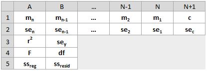
These statistics may be described as follows:
| Statistic | Description |
|---|---|
se1, se2, …, sen | The standard error is a measure of the statistical accuracy of an estimate, equal to the standard deviation of the theoretical distribution of a large population of such estimates. It is usually estimated in practice as the sample standard deviation divided by the square root of the sample size (assuming statistical independence of the values in the sample), |
| seb | Standard error value for the constant c (but this is equal to #N/A when constant is FALSE |
| r2 | This the coefficient of determination, which compares estimated and actual y-values and ranges, with a value between zero(0) and one (1). If it is 1, there is a perfect correlation in the sample, i.e. there is no difference between the estimated y-value and the actual y-value. At the other extreme, if the coefficient of determination is zero, the regression equation is not helpful in predicting a y-value. The coefficient of determination, R2, is the proportion of the variance in the dependent variable that is predictable from the independent variable(s). There are several definitions of R2, but they are not always equivalent (indeed, they can be negative on ocassion). One class of such cases includes that of simple linear regression where r2 is used instead of R2. When an intercept is included, then r2 is simply the square of the sample correlation coefficient (i.e. r) between the observed outcomes and the observed predictor values. Here, the coefficient of determination will range between zero (0) and one (1) |
| sey | Standard error for the y estimate |
| F | This is the F statistic or the F-observed value. You should use the F statistic to determine whether the observed relationship between the dependent and independent variables occurs by chance This may be calculated using the F.INV.RT function in Excel. An F statistic is a value you get when you run an analysis of variance (ANOVA) test or a regression analysis to find out if the means between two populations are significantly different. It’s similar to a T statistic from a T-Test: a T-test will tell you if a single variable is statistically significant, whereas an F test will tell you if a group of variables are jointly significant |
| df | The degrees of freedom. You should use the degrees of freedom to help you find F-critical values in a statistical table. Compare the values you find in the table to the F statistic returned by LINEST to determine a confidence level for the model. The degree(s) of freedom is the number of independent values or quantities which may be assigned to a statistical distribution. It is is calculated as follows. When no x columns are removed from the model due to collinearity: if there are k columns of known_x’s and constant = TRUE or is omitted, df = n – k – 1 if constant = FALSE, df = n - k In both cases, each x column that is removed due to collinearity increases the value of df by one (1) |
| ssreg | This is the regression sum of squares In regression analysis, Excel calculates for each point the squared difference between the y-value estimated for that point and its actual y-value. The sum of these squared differences is called the residual sum of squares, ssresid. Excel then calculates the total sum of squares, sstotal. When the constant argument = TRUE or is omitted, the total sum of squares is the sum of the squared differences between the actual y-values and the average of the y-values. When the constant argument = FALSE, the total sum of squares is the sum of the squares of the actual y-values (without subtracting the average y-value from each individual y-value). Then, the regression sum of squares, ssreg, may be found from: ssreg = sstotal - ssresid. The smaller the residual sum of squares is, compared with the total sum of squares, the larger the value of the coefficient of determination, r2, which is an indicator of how well the equation resulting from the regression analysis explains the relationship among the variables. The value of r2 equals ssreg/sstotal |
| ssresid | This is the residual sum of squares, as explained above. |
To be clear:
- you can describe any straight line with the slope and the y-intercept:
o slope (m): to find the slope of a line, often written as m, take two points on the line, (x1, y1) and (x2, y2); the slope is equal to (y2 - y1)/(x2 - x1)
o y-intercept (c): the y-intercept of a line, often written as c, is the value of y at the point where the line crosses the y-axis.
o the equation of a straight line is given by y = mx + c. Once you know the values of m and c, you can calculate any point on the line by plugging the y- or x-value into that equation. You may also use the TREND function
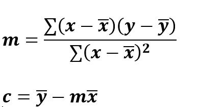
- when you have only one independent x-variable, you can obtain the slope and y-intercept values directly by using the following formulae:
o slope: =INDEX(LINEST(known_y's, known_x's), 1)
o y-intercept: =INDEX(LINEST(known_y's, known_x's), 2)
- the accuracy of the line calculated by the LINEST function depends upon the degree of scatter in your data. The more linear the data, the more accurate the LINEST model will be. LINEST uses the method of least squares for determining the best fit for the data. When you have only one independent x-variable, the calculations for m and c are based on the following formulae:·
- the line- and curve-fitting functions LINEST and LOGEST can calculate the best straight line or exponential curve that fits your data. However, you have to decide which of the two results best fits your data. You can calculate TREND(known_y's, known_x's) for a straight line, or GROWTH (known_y's, known_x's) ues predicted along that line or curve at your actual data points. You can then compare the predicted values with the actual values. You may want to chart them both for a visual comparison
- in some cases, one or more of the x columns (assume that y’s and x’s are in columns) may have no additional predictive value in the presence of the other X columns. In other words, eliminating one or more x columns might lead to predicted y values that are equally accurate. In that case, these redundant x columns should be omitted from the regression model. This phenomenon is called collinearity because any redundant x column can be expressed as a sum of multiples of the non-redundant x columns. The LINEST function checks for collinearity and removes any redundant x columns from the regression model when it identifies them. Removed X columns can be recognised in LINEST output as having zero (0) coefficients in addition to zero (0) se values. If one or more columns are removed as redundant, df is affected because df depends upon the number of x columns actually used for predictive purposes
- if df is changed because redundant x columns are removed, values of sey and F are also affected. Collinearity should be relatively rare in practice. However, one case where it is more likely to arise is when some x columns contain only zero (0) and one (1) value as indicators of whether a subject in an experiment is or is not a member of a particular group. If constant = TRUE or is omitted, the LINEST function effectively inserts an additional x column of all one values to model the intercept. If you have a column with a 1 for each subject if male, or 0 if not, and you also have a column with a 1 for each subject if female, or 0 if not, this latter column is redundant because entries in it can be obtained from subtracting the entry in the “male indicator” column from the entry in the additional column of all 1 values added by the LINEST function
- formulae that return arrays must be entered as array formulas; however, do note that in Excel for the web you cannot create array formulae
- when entering an array constant (such as known_x's) as an argument, use commas to separate values that are contained in the same row and semicolons to separate rows. Separator characters may be different depending on your regional settings
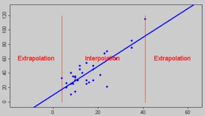
- note that the y-values predicted by the regression equation may not be valid if they are outside the range of the y-values you used to determine the equation (i.e. extrapolation versus interpolation)
- In addition to using LOGEST to calculate statistics for other regression types, you can use LINEST to calculate a range of other regression types by entering functions of the x and y variables as the x and y series for LINEST. For example, the following formula:
=LINEST(yvalues, xvalues^COLUMN($A:$C))
works when you have a single column of y-values and a single column of x-values to calculate the cubic (polynomial of order three [3]) approximation of the form:
y = m1x + m2x2 + m3x3 + c
You can adjust this formula to calculate other types of regression, but in some cases it requires the adjustment of the output values and other statistics
- The F-test value that is returned by the LINEST function differs from the F-test value that is returned by the FTEST function. LINEST returns the F statistic, whereas FTEST returns the probability.
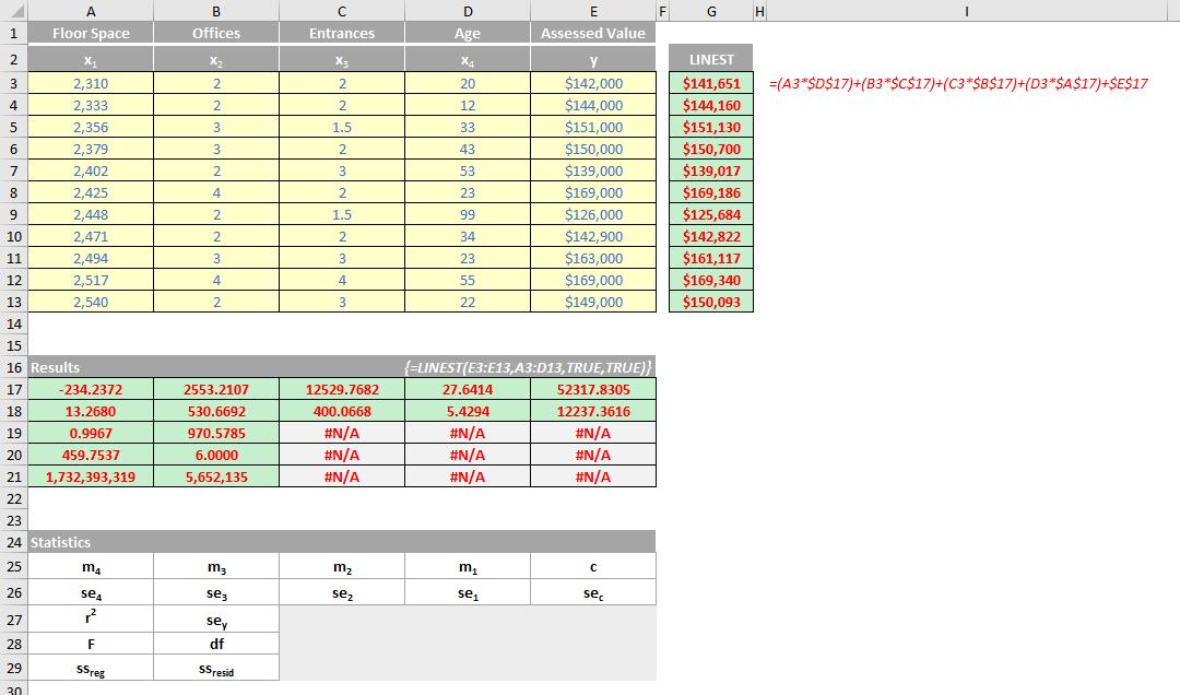
Please see my comprehensive example below:
We’ll continue our A to Z of Excel Functions soon. Keep checking back – there’s a new blog post every business day.
A full page of the function articles can be found here.