
Monday Morning Mulling: July 2021 Challenge
2 August 2021
On the final Friday of each month, we set an Excel / Power Pivot / Power Query / Power BI problem for you to puzzle over for the weekend. On the Monday, we publish a solution. If you think there is an alternative answer, feel free to email us. We’ll feel free to ignore you.
This month, we wanted you to check out our model or else check out (did my checkout joke register?). [Please stop – Ed.]
The Challenge
This month, we provided a link to a model for you to peruse:
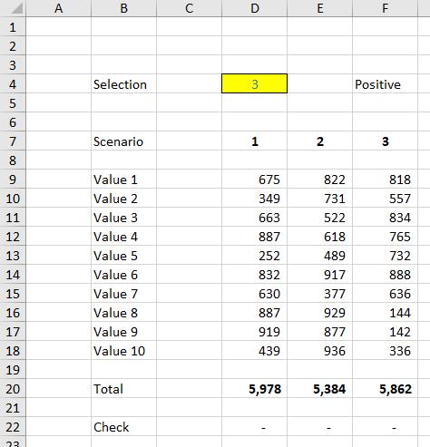
It was not the world’s most complex workbook but it did contain the odd problem. How many did you spot?
Suggested Solution
It seems a very simple model, but I may have been a little devious – all may not be quite as it seems. For a start, did you notice what happens when you open the file?
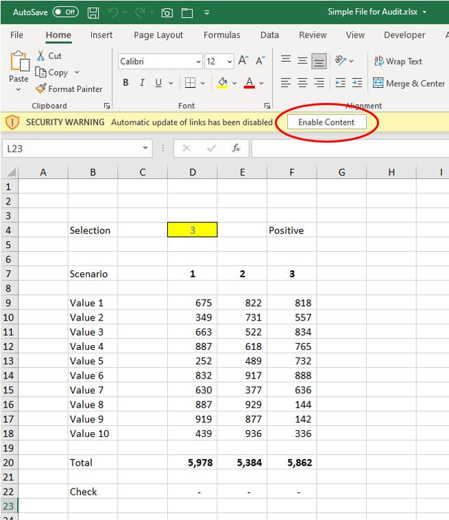
Many fail to notice the yellow bar that pops up between the Ribbon and the Formula bar. For some that do, they believe it to be a prompt for enabling macros as the button says, ‘Enable Content’. But it isn’t. It is highlighting the model contains links to another workbook. As reviewers we need to know: is this link / are these links intentional? The only way to answer that is to locate them.
But wait, Liam, I don’t see the message at all. I didn’t know there were any links!
Watch out.
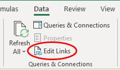
On the ‘Data’ tab of the Ribbon, click on ‘Edit Links’ (ALT + E + K), viz.
This results I the following ‘Edit Links’ dialog if and only if there are any links!
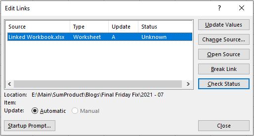
Clearly, there are links – so if the message did not display for you, check out the ‘Startup Prompt…’ button in the bottom left-hand corner. Clicking on this may prove insightful:
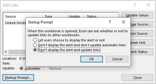
Hmmm… that’s interesting! Somebody has gone to great pains to hide the fact there are links in this model. I would imagine most expert users of Excel would not be aware of this wonderful little feature.
Now I’m worried. What is this link?
You can choose to ‘Break Link’ (remember: link implies there is only one workbook linked, no that it is only one link), which effectively takes all formulaic links and copies and pastes them as values. The problem is, you’ll be none the wiser as to what the link was and why it was there.
To search for links, the most common approach is to call the Find dialog (CTRL + F):
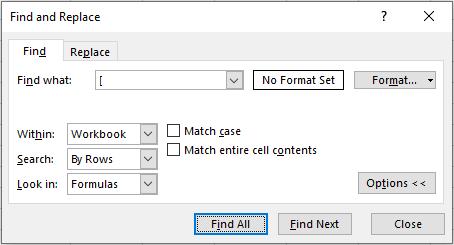
Links to other workbooks always contain open and closed square brackets, so clicking on the ‘Options‘ button and searching looking for Formulas in the entire Workbook for ‘[‘ will find any formulaic links. Unfortunately:
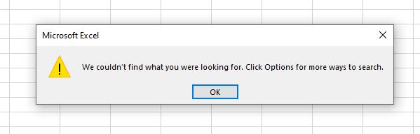
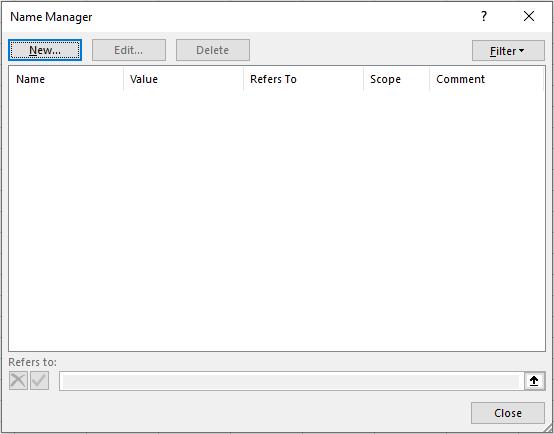
Trying all options will reveal nothing. Indeed, Formula Manager (CTRL + F3) – another common place where links hide out – reveals even less:
And the award for the most useless graphic in a blog goes to the above image. Congratulations.
So at least we are no errors in range names. There aren’t any. So where is this pesky link? Chasing so-called “phantom links” is the bane of many a modeller and indeed, we have written Thought articles on this phenomenon previously (such as Locating Links and the even more cleverly-titled Locating Links #2 ). It turns out we have an object link.
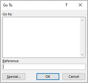
To hunt out objects, open the ‘Go To’ dialog (F5) (or Home -. Find & Select -> Go To…):
Click on the ‘Special…’ button in the bottom left-hand corner:
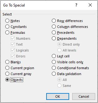
Clicking on ‘Objects’ in the bottom left-hand corner and clicking ‘OK’ reveals the following little stowaway:
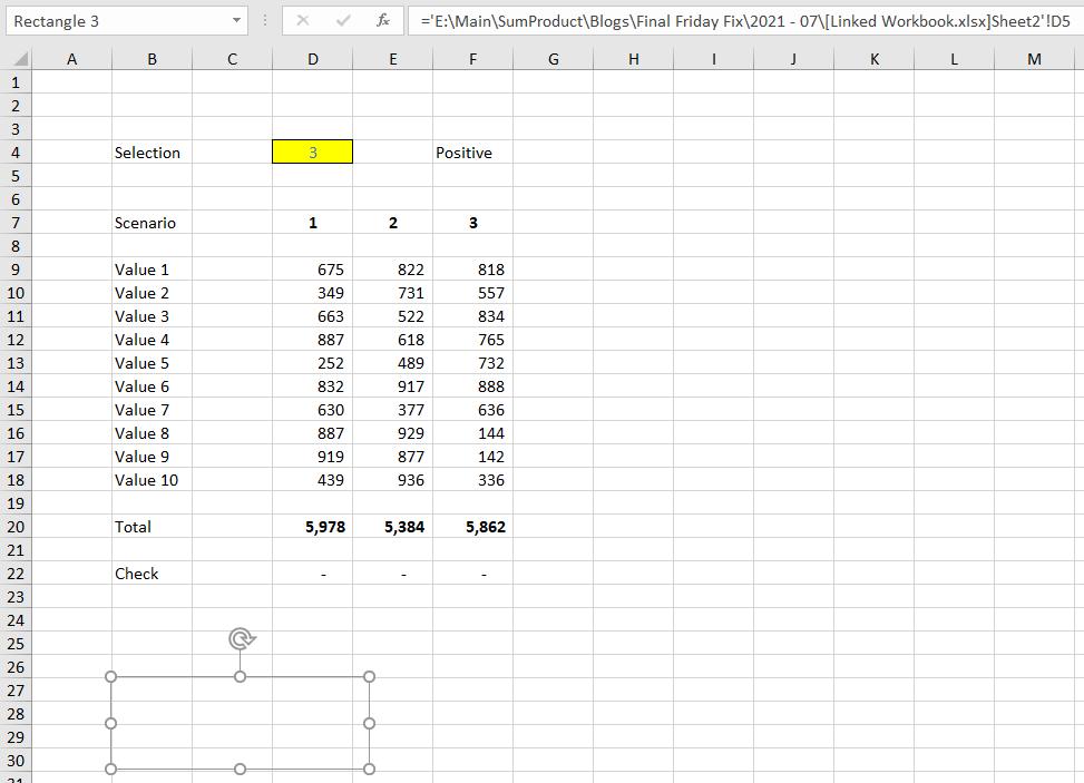
Pesky little critter. Someone has added a hidden object that contains a formula (see Formula bar) that links to that other workbook. Clearing the Formula bar or deleting the rectangle will remove the link. Note this shape is called ‘Rectangle 3’ (check the Name Box), but it did not appear in the Name Manager dialog. Excel can be frustrating sometimes.
OK, now that’s dealt with; let’s take a look at what we have:
Take a look at the horizontal and vertical scrollbars. It’s a dead giveaway that all is not as it seems when the positional blocks are so small – it means the spreadsheet is large. The keyboard shortcut CTRL + END will take you to the last used column and last used row of this worksheet:
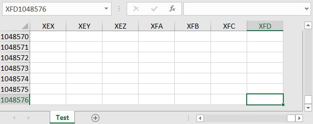
XFD1048576 – which in fact contains a blank space! It should be noted that the cell you are taken to often contains nothing: it merely represents the intersection of the final row and final column used, so you may need to look above (CTRL + Up Arrow) and to the left (CTRL + Left Arrow).
Deleting the contents will not reset the positional blocks: you will need to save the file, close and re-open to achieve that result.
But there was an easier way to identify these issues. Did you go here?
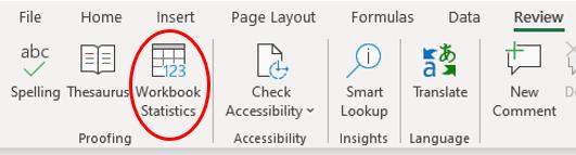
On the Review tab of the Ribbon, click on ‘Workbook Statistics”:
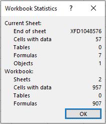
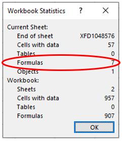
This helpful dialog reveals the last cell, observes there is an object and that there are 907 formulae in total. Sorry – where!?
That doesn’t look like 907 formulae to me. That’s because there are only seven [7] on this worksheet, but there is another sheet (the dialog states there are two [2]). OK, where?

There is only one visible sheet. It must be hidden. If we right-click on the sheet tab:
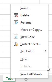
‘Unhide…’ is greyed out indicating there are no hidden sheets. But there must be. So where the heck is it? To locate it, we need to open the Visual Basic Editor (ALT + F11):
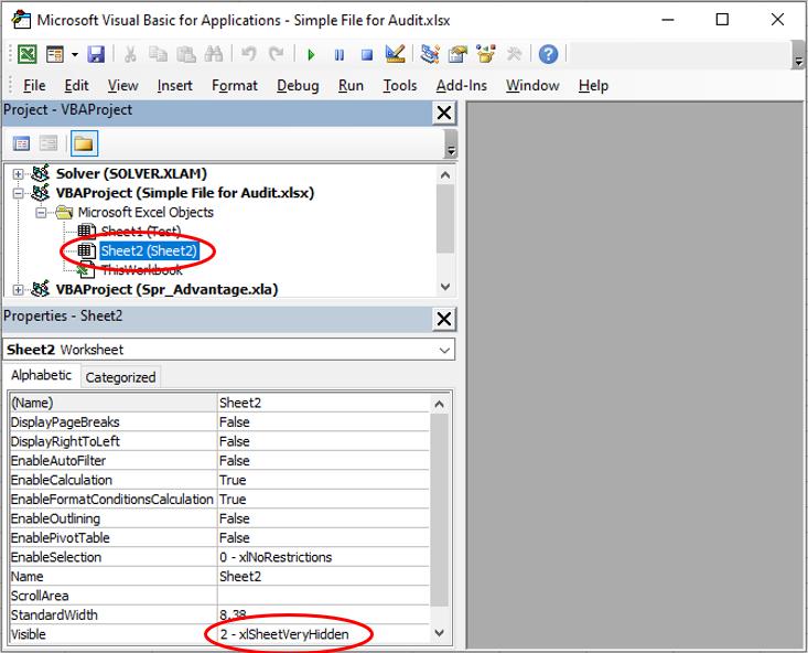
From the image above, you can spot Sheet2 (cunningly called ‘Sheet2’) and it is “Very Hidden”, just like Microsoft’s grasp of grammar. If we change the ‘Visible’ property to ‘-1 – xlSheetVisible’, the sheet will appear once the Visual Basic Editor has been closed:
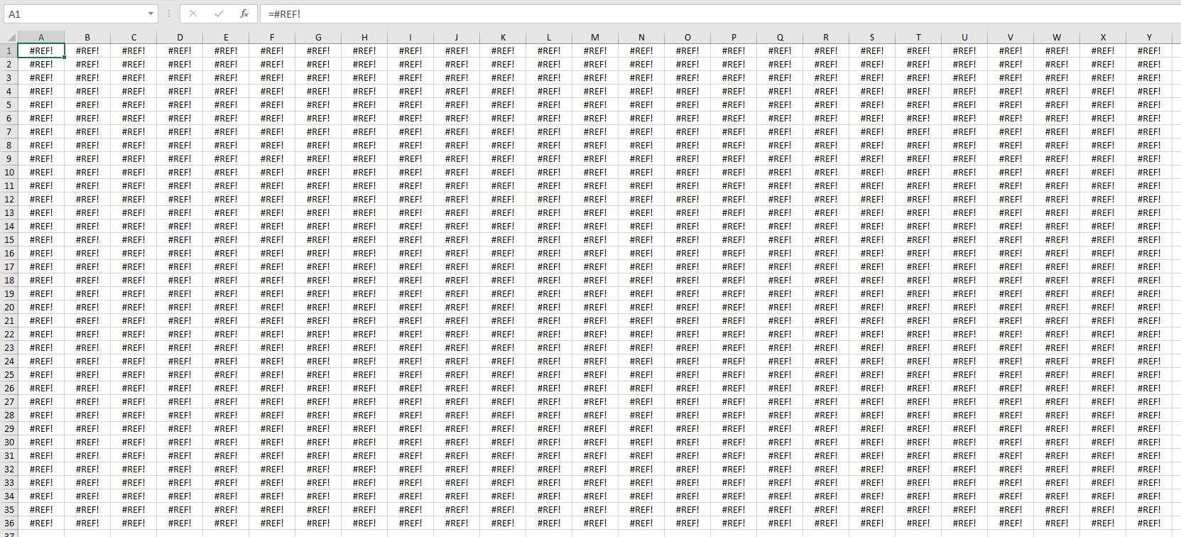
Did you spot these errors..?
Clearly, it is best to use Excel’s resources wherever you can to assist you. The Formulas (sic) tab has a useful feature, namely ‘Error Checking’:
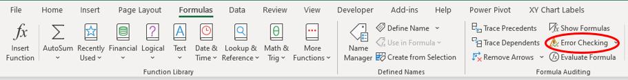
However, clicking this button in this instance reveals nothing:
But it is always worth a shot!
From earlier, we know there are only seven formulae to review on this worksheet:
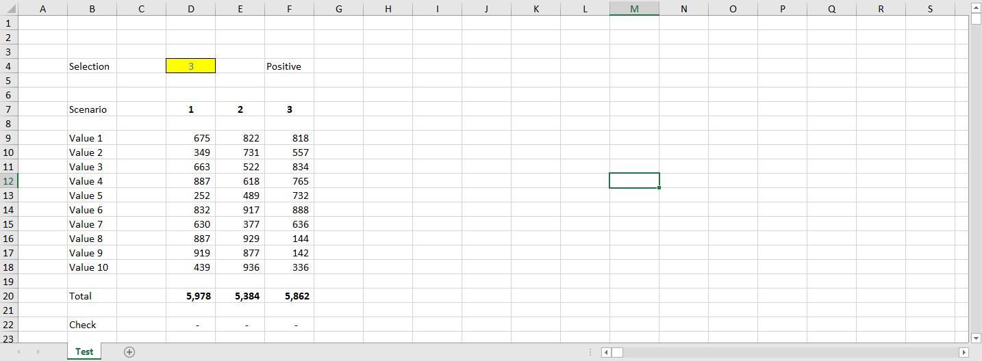
There are various ways to locate the seven. One is to use Go To -> Special again and select Formulas (sic):
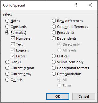
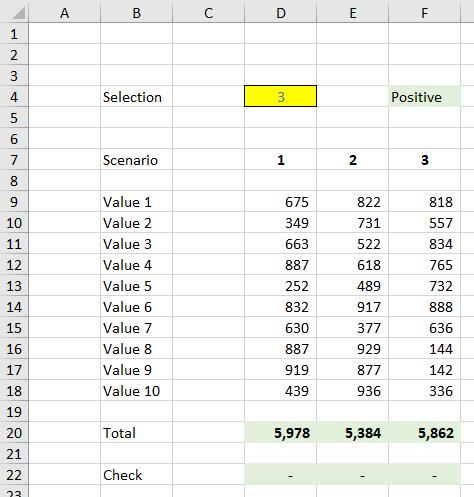
Once you click on ‘OK’, the seven are revealed (highlighted in green, below):
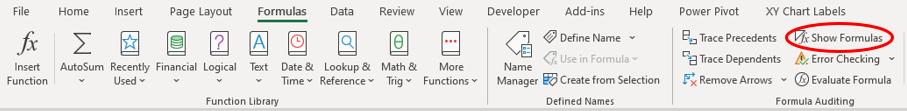
Alternatively, the formulae may be displayed using Formulas -> Show Formulas (or CTRL + `):
This will reveal the following:
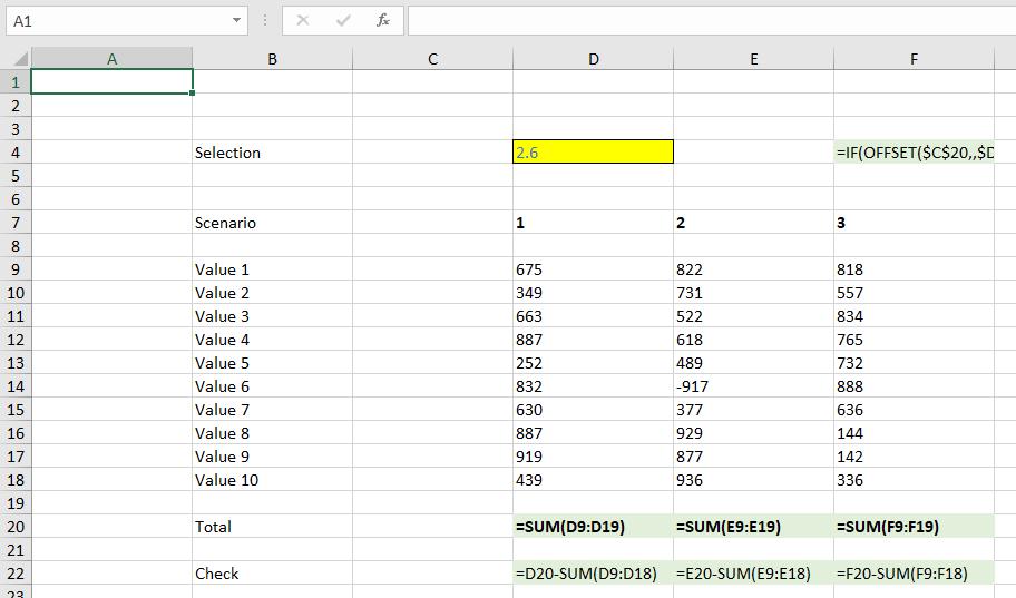
Either by inspection (or by using CTRL + \), it’s clear that there are only three unique formulae (i.e. formulae that are not copies of other formulae), namely in cell F4, D20 and D22.
The formula in cell F4 is given by
=IF(OFFSET($C$20,,$D4)>0,"Positive","Negative")
This is wrong, but is probably our first issue that may be unintentional. The first part of this IF statement tests whether some calculation is positive. If it is, the result is “Positive”. That’s fine. However, it otherwise returns “Negative” – but what if the result is an error or zero? Neither of these are negative values. The logic should be better defined.
The formula in D20 may give rise to a problem too:
=SUM(D9:D19)
Note that row 19 is a blank row. You should never refer to unprotected blank rows in formulae because end users have an annoying habit of typing things in blank cells. This could cause an issue, but at least the formula in cell D22 would alert you:
=D20-SUM(D9:D18)
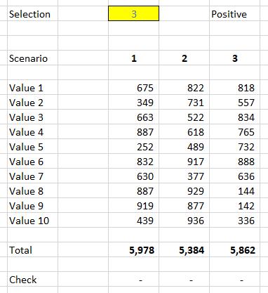
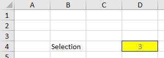
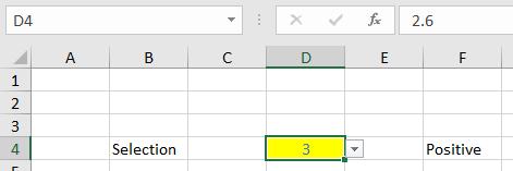
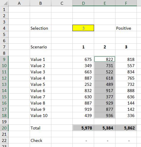
It seems we are finished – except we aren’t. Did you notice how the value in cell D4 changed when you toggled between the normal view and showing formulae? Originally it displayed ‘3’:
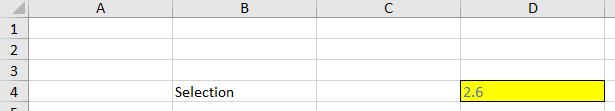
But then it showed ‘2.6’:
How does that happen?
A closer inspection of the Formula bar shows the value was always ‘2.6’:
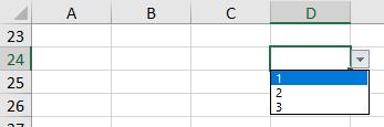
So why does it show ‘3’? Number formatting will not explain this as this would not change when you ‘Show Formulas’. Note instead that the cell contains data validation (ALT + D + L or Data -> Data Validation):
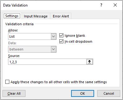
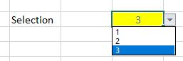
This cell has been validated to contain a drop down list of the numbers 1, 2 and 3:
However, a little known bug in Excel allows values between 1 and 3 to be allowed here in certain circumstances – which has what has happened here. This could cause issues for our formula in cell F4, for example. Another sneaky issue.
It might be best to check there is no more data validation in the workbook using F5 -> Special once more:
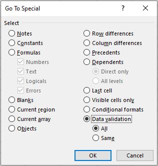
This reveals an erroneous drop down list in cell D24:
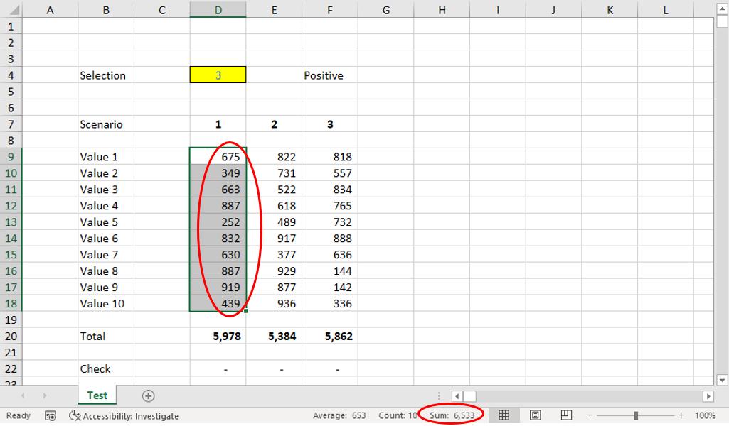
Surely there is nothing else in such a simple model, yes? Given the issues identified, it might be best to check those sums manually. You can do this by highlighting the values and then checking the summation in the status bar. For example:
What!?
- Column D totals 6,533 not 5,978
- Column E totals 5384 (correct)
- Column F totals 5,852 not 5,862
Hang on, we have checked the formulae (row 20) and the Check (row 22). How can these errors occur? Number formatting of cell D20 reveals something rather interesting:
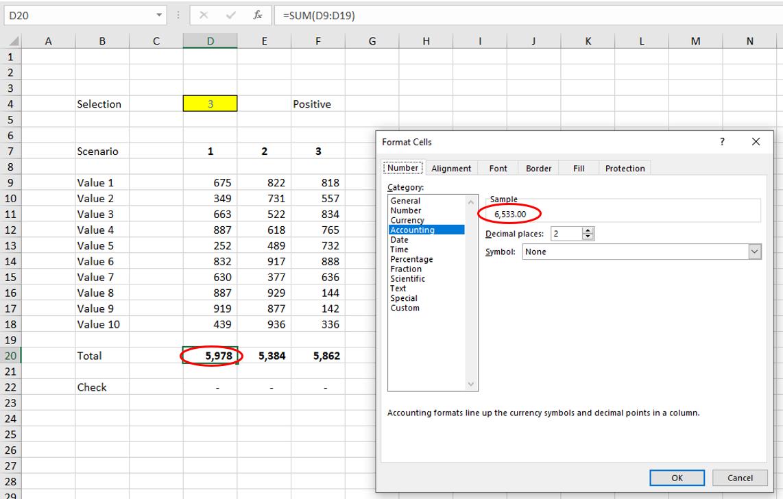
How can the sample in the ‘Format Cells’ dialog show the value as ‘6,533.00’ yet it is displayed as ‘5,978’ in cell D20 and the error check in cell D22 is not triggered? Has someone been up to no good with conditional formatting..?
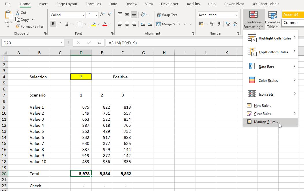
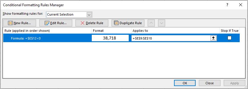
Going to Home -> Conditional Formatting -> Manage Rules… (ALT + O + D):
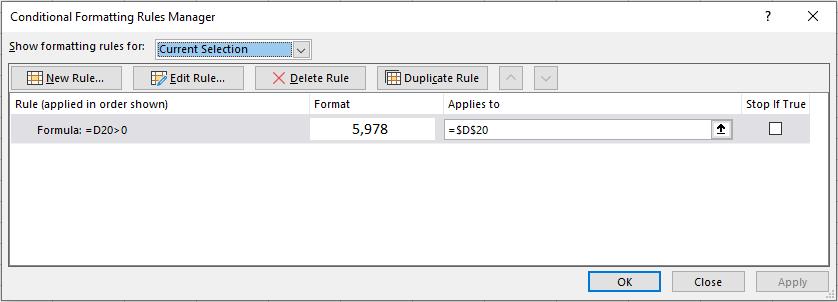
That’s more like it. The format is ‘5,978’ apparently. If you ‘Edit Rule…’ and go to the Number tab of the resulting (conditional) ‘Format Cells’ dialog, the cell’s murky secret is finally revealed:
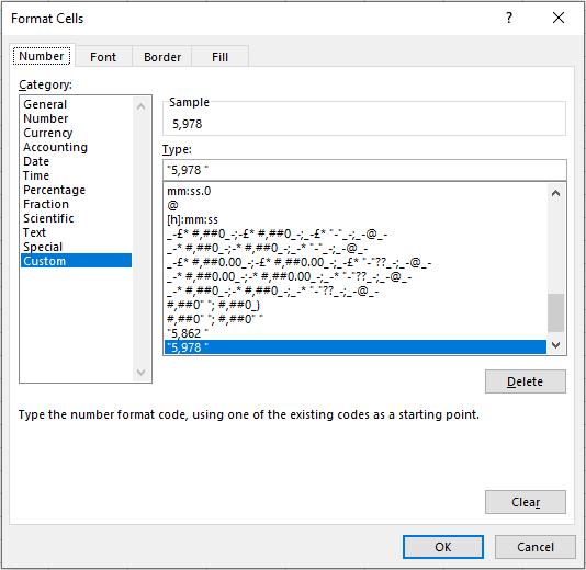
All numbers have been made to appear as ‘5,978’. That’s fraud – especially given how deep this deviation is buried. Let’s be honest, how many of you spotted this?
A similar issue may be identified in cell F20. At least the modeller had the decency to leave cell E20 alone! I suppose we had better check to see if there is any more crafty conditional formatting prevalent in this worksheet. For a final time, F5 -> Special comes to the rescue, viz.
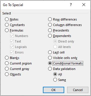
Once ‘OK’ is pressed, there is an interesting revelation:
Column E’s inputs and the formula in cell E20 have all been conditionally formatted. Following the steps from above, we identify the following for all of the Column E cells:
Format ’38,718’? None of the numbers show this value. What’s happened this time?
It appears ’38,718’ must be Excel “code” for certain types of “common” number formatting (to be honest, I am merely speculating here). The conditional number formatting identifies the following for cell E9:
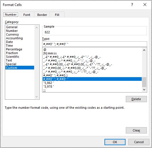
These cells contain the following conditional custom number format:
#,##0" "; #,##0" "
We have talked about custom number formatting before. This syntax means “show positive AND negative numbers as positive numbers”. Adding a space to the end merely makes the numbers appear formatted similar to the numbers in columns D and F – further evidence the modeller is intending to be sneaky.
Therefore, the total in column E may be correct, but the values in cells E8:E18 may be misleading. Indeed, as a simple check,
822 + 731 + 522 + 618 + 489 + 917 + 377 + 929 + 877 + 936 = 7,218
Last time I checked 7,218 is not equal to 5,384! (And no, I don’t mean factorial…) The value in cell E14 is actually minus 917, not 917 – hence the difference of 1,834 (= 917 - -917).
So how did you do? Did you get them all? If you did, I suspect you are someone who should have their spreadsheets checked!
Word to the Wise
The above was only meant to be a bit of fun, but it does highlight the importance of checking a model – and it may also have drawn your attention to the difference between an honest mistake (clanger) and something much more worrying: the intention to deceive, i.e. fraud.
Model reviewers / auditors are often referred to as “watchdogs, not bloodhounds”. Fraud is fraud: that is, the author is intending to mislead. Tricks may be elaborate and you cannot expect a model reviewer / auditor to find all (any?) such issues, merely that they follow industry standard appropriate checks of review.
And the problem is presently, no such standard exists.
The comment in the Final Friday Fix may have been flippant in its introduction regarding the document How to Review a Spreadsheet, but hopefully this month’s Fix shows the bar should be set relatively high and perhaps should be “Fixed”. The problem is experts cannot agree. What a happy note to end on.
Until next month!
The Final Friday Fix will return on Friday 27 August 2021 with a new Excel Challenge. In the meantime, please look out for the Daily Excel Tip on our home page and watch out for a new blog every business workday.