
Monday Morning Mulling: August 2023 Challenge
28 August 2023
On the final Friday of each month, we set an Excel / Power Pivot / Power Query / Power BI problem for you to puzzle over for the weekend. On the Monday, we publish a solution. If you think there is an alternative answer, feel free to email us. We’ll feel free to ignore you.
The challenge this month was to find favourite stores and most recently visited stores by customer from sales data, using only one [1] Excel formula for each task.
The Challenge
Last Friday, we challenged you to find out the favourite store of each customer using only one [1] Excel formula, and to find the last store that each customer visited with, again, “just” one [1] formula. You could download the question file here.
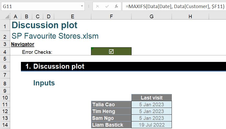
The table Data contained the customer visits data, and the desired outputs were to look like the following upon completion:
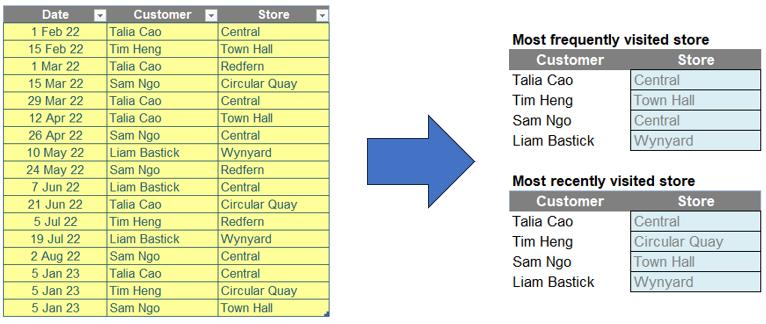
There were some requirements:
- each formula needed to be within one cell
- this was a formula challenge; no Power Query / Get & Transform or VBA.
Suggested Solution for Task 1: Most
Frequently Visited Store
You can find our Excel file here, which shows our suggested solution. The steps are detailed below.
COUNT THE VISITS
We can begin by using UNIQUE and TRANSPOSE to get the lists of customers and stores from Data, and place them as row and column headers for our array of counts. The formula
=UNIQUE(Data[Customer])
provides an unsorted list of the customers down a column. The formula
=TRANSPOSE(UNIQUE(Data[Store]))
provides a list of the stores across a row (hence the need for the TRANSPOSE function, which transforms a column vector to a row vector).
The number of visits by customer to a store can be found using COUNTIFS with Data[Store] and Data[Customer] as the criteria ranges. Also, be careful with table references and remember to use CTRL + D and CTRL + R to copy the formula down and to the right. Then COUNTIFS produces the following matrix of counts:
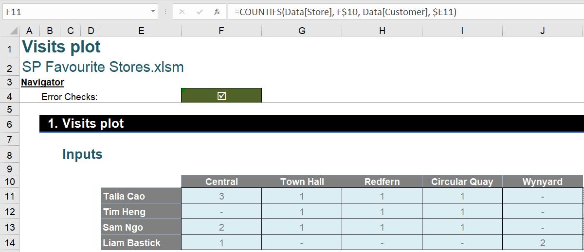
Moreover, if we use the column headers (stores) in the first criteria argument of COUNTIFS instead of single stores, and the row headers (customers) in the second criteria argument, we can obtain the whole matrix as a spilled array using only one formula:
=COUNTIFS(Data[Store], F10#, Data[Customer], E11#)
This is the Dynamic Array equivalent of a PivotTable.
FIND THE FAVOURITE STORES
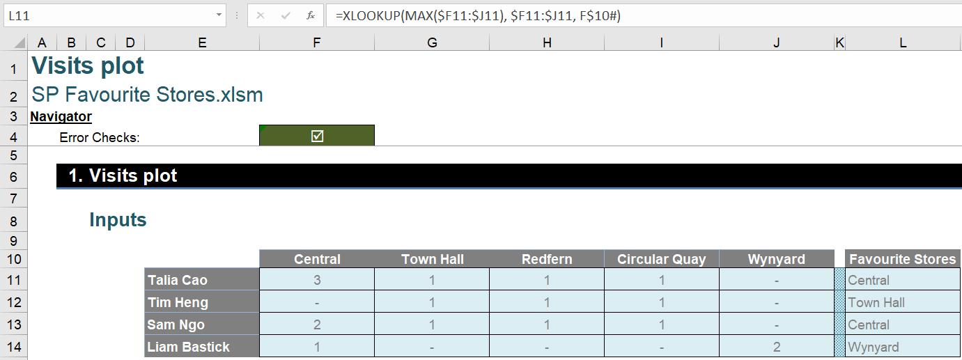
Given the matrix of visit counts, we can look for the most frequently visited store by each customer and output the corresponding store name. An XLOOKUP formula for the maximum of each row with store names being the return array can achieve that:
=XLOOKUP(MAX($F11:$J11), $F11:$J11, F$10#)
Here it’s necessary to anchor the column titles F10# at the row, to fill down for all customers. The output would look like the following:
So how do we look up for all customers in one [1] formula? We can use the BYROW function. The BYROW function has two [2] arguments: an array and a LAMBDA function:
=BYROW(array, LAMBDA(parameter, calculation))
The LAMBDA function takes each row of the array as its parameter and performs the specified calculation on it. Given the above matrix F11# of visit counts, we can use a BYROW function on the whole matrix, and write the XLOOKUP as the LAMBDA function inside:
=BYROW(F11#, LAMBDA(r, XLOOKUP(MAX(r), r, F10#)))
Then, the XLOOKUP will be performed row-by-row (hence the name BYROW). For interested readers we have written blogs with more details on BYROW and LAMBDA.
COMBINE THE FORMULAE
In the previous two [2] steps, we first obtained the matrix F11# of visit counts using COUNTIFS with two-dimensional conditions, and then we used BYROW on F11# to perform an XLOOKUP for the most frequently visited store by each customer. The two [2] steps can be combined by writing the first formula in place of F11# inside the second formula:
=BYROW(COUNTIFS(Data[Store], F10#, Data[Customer], E11#),
LAMBDA(r, XLOOKUP(MAX(r), r, F10#)))
The COUNTIFS matrix is only a helper, so instead of referencing the column headers (F10#) and row headers (E11#), we can substitute with the original UNIQUE and TRANSPOSE formulas:
=BYROW(COUNTIFS(Data[Store],
TRANSPOSE(UNIQUE(Data[Store])),
Data[Customer], UNIQUE(Data[Customer])),
LAMBDA(r, XLOOKUP(MAX(r), r, TRANSPOSE(UNIQUE(Data[Store])))))
For better readability, we can also use a LET function to name some variables for intermediate steps:
=LET(Store, TRANSPOSE(UNIQUE(Data[Store])),
Customer, UNIQUE(Data[Customer]),
Matrix, COUNTIFS(Data[Store], Store, Data[Customer], Customer),
BYROW(Matrix, LAMBDA(r, XLOOKUP(MAX(r), r, Store))))
Here we name the intermediate matrix Matrix, and the final calculation of the LET is a BYROW on Matrix to look-up the MAX from each row.
Suggested Solution for Task 2: Most Recently Visited Store
You can find our Excel file here which demonstrates our suggested solution.
STARTING SIMILARLY…
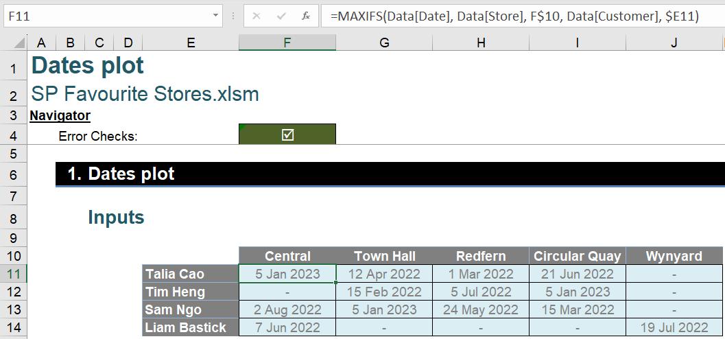
To find the lastly visited store by each customer, we can use an approach very similar to the previous solution, by sorting visit dates of each customer to each store with a MAXIFS:
=MAXIFS(Data[Date], Data[Store], F$10, Data[Customer], $E11)
Again, use CTRL + D and CTRL + R to fill the formula down and to the right. Then the output will look like the following:
We can look up the latest visit of each customer to return the corresponding store. Furthermore, following the same process we can build up a final formula:
=LET(Store, TRANSPOSE(UNIQUE(Data[Store])),
Customer, UNIQUE(Data[Customer]),
Matrix, MAXIFS(Data[Date], Data[Store], Store, Data[Customer], Customer),
BYROW(Matrix, LAMBDA(r, XLOOKUP(MAX(r), r, Store))))
A DIFFERENT APPROACH
The above approach is arguably not optimal for the second task, in the sense that it is sorting dates twice. The MAXIFS first sorts visit dates for each customer to each store, and then the XLOOKUP sorts the latest visits to each store by each customer. Conceptually, the optimal algorithm would be sorting all visits of each customer by dates, and then returning the corresponding stores of those latest visits. That is, instead of a two-dimensional problem, this task is a two-layer problem.
We can use the combination of FILTER, SORT and INDEX. For example, for the customer ‘Sam Ngo’, we can get his most recently visited store with the following formula:
=INDEX(SORT(FILTER(Data, Data[Customer] = "Sam Ngo"), 1, -1), 1, 3)
Here FILTER first filters for all store visits of this customer. Then SORT sorts the first column, Date, in descending order, so the first row of the spilled array will contain the date, customer name and the store location of the latest store visit of ‘Sam Ngo’. Lastly INDEX outputs the cell in the first row and the third column (Store) of the table.
To cover all customers in one formula, we can again use BYROW:
=BYROW(UNIQUE(Data[Customer]), LAMBDA(name, INDEX(SORT(FILTER(Data, Data[Customer]=name), 1, -1), 1, 3)))
COMPARING THE APPROACHES
The advantage of the above approach is that FILTER preserves rows of the table Data. Consider instead if we were to use MAXIFS instead of FILTER and SORT, to replicate the same idea of sorting Date for each Customer first and then return the corresponding Store. For each customer we would start with:
=MAXIFS(Data[Date], Data[Customer], $F11)
Then the outcome would be a single date value, which is not necessarily unique:
That means we can’t use the sorted-out dates alone to look up the corresponding Store. We have no choice but to combine it with the list of customers. One way is to use the ampersand (&) to concatenate a unique Customer-Date label, to look up from the table Data:
=INDEX(Data[Store], MATCH($F11&" – "&$G11,
Data[Customer]
&" – "&Data[Date], 0))
In comparison, FILTER preserves the rows, and hence preserves the Date-Customer-Store connection. We just need to specify the index to sort and to output.
The Final Friday Fix will return on Friday 29 September 2023 with a new Excel Challenge. In the meantime, please look out for the Daily Excel Tip on our home page and watch out for a new blog every business working day.