
Monday Morning Mulling: February 2018 Challenge
26 February 2018
Last week, we asked how you could set up a cell to pick up text from parts of an Excel spreadsheet, and present it in a ready-for-email form.
While there are a few ways, here’s one that we think should be sufficiently easy to implement.
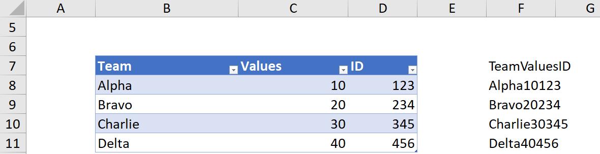
To make it easier to follow, we’ve created a new column off to the right with the following formula:
=Table1[@Team]&CHAR(9)&CHAR(9)&Table1[@Values]&CHAR(9)&CHAR(9)&Table1[@ID]
The “CHAR(9)” bit is the key thing – each effectively adds a tab space between the different values in the table. This allows us to get a consistently sized space between each part of the table. We can also add a similar formula to get the header labels:
=Table1[[#Headers],[Team]]&CHAR(9)&CHAR(9)&Table1[[#Headers],[Values]]&CHAR(9)&CHAR(9)&Table1[[#Headers],[ID]]
Note that when displayed in Excel, the tab spaces don’t show up in the text string. Never mind that though, we’ll see it soon enough.
The final step is to bring these values into the target cell. We can do this using the following formula:
=C4&CHAR(10)&CHAR(10)
&F7&CHAR(10)
&F8&CHAR(10)
&F9&CHAR(10)
&F10&CHAR(10)
&F11&CHAR(10)
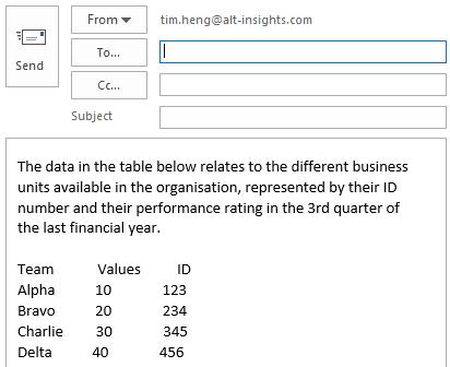
This combines the opening statement in C4, and adds extra lines using the CHAR(10) code, which creates a new line in the text string. This gives me an email that looks like this:
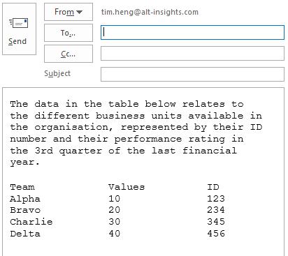
Finally, in order to line up the column values, I can change the font to a monospaced one, such as Courier New, which results in this final email:
There you have it! While you can use vbNewLine and vbTab in VBA to do something similar, this is how you can perform the equivalent tasks in Excel.
Join us again on the last Friday of March for our next Final Friday Fix!