
Power Query: Three Sheets to the Table
9 June 2021
Welcome to our Power Query blog. This week, I look at combining sheets where the columns do not match.
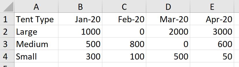
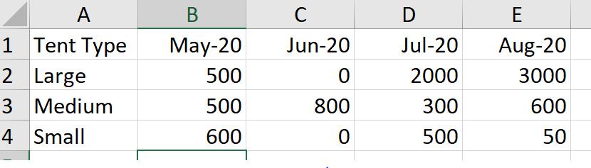
I have some data that has come in from John, one of my imaginary salespeople. He has sent in some sales data, and I need to pull it into one table. The data is spread over three sheets, which are all in a similar format:
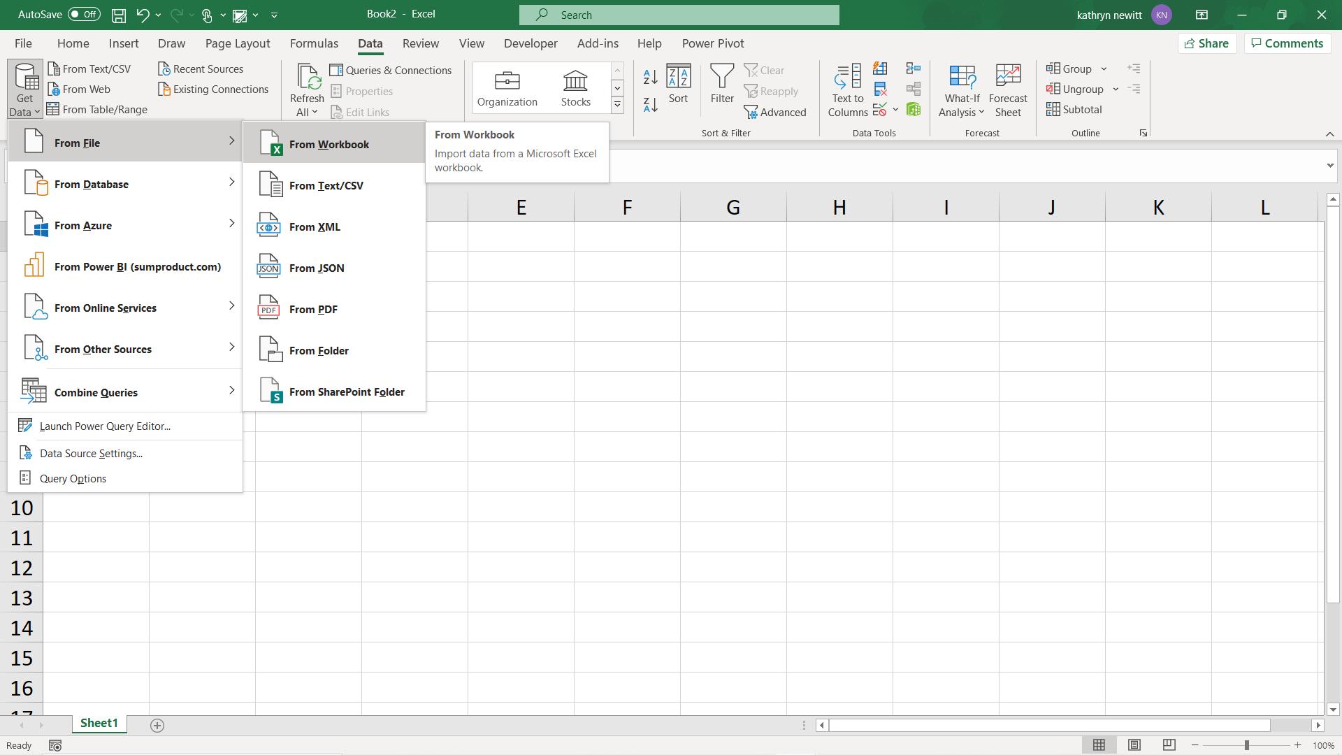
In my (new) Excel workbook, I go to the Data tab and choose to ‘Get Data’ and then ‘From Workbook’, viz.
This allows me to see the data in John’s workbook:
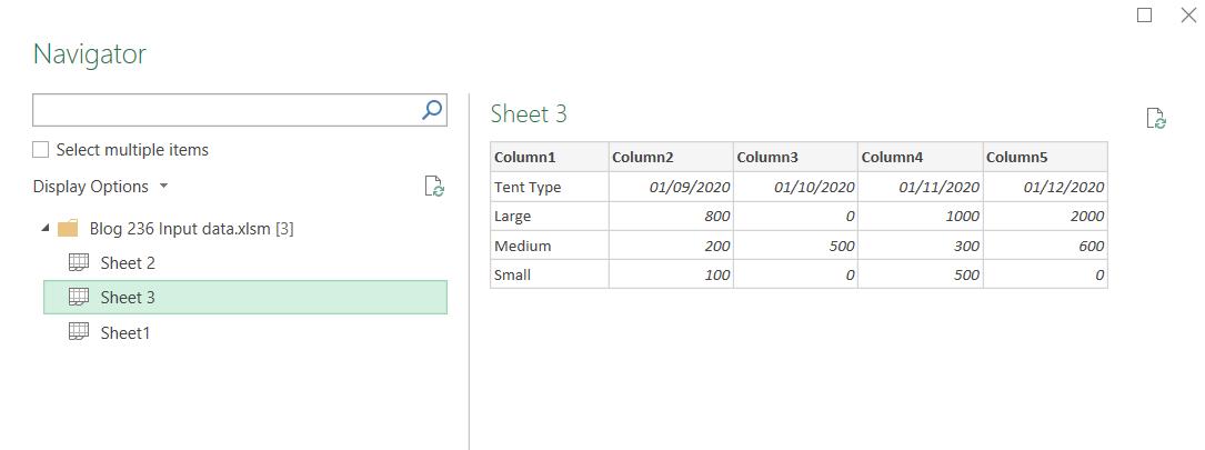
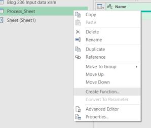
Because the columns are not the same for each sheet, if I tried to append my sheets, I would end up with the dates in the middle of my data, which is not what I want. I need to transform each sheet before I combine them. However, there is another option I can take if I right-click on the workbook:
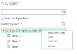
I can transform the data in the workbook. I select this option.
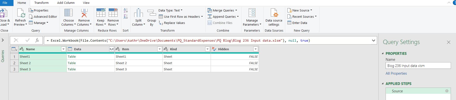
This gives me the source step (I know I could have chosen sheets and deleted steps to get to this point, but this is neater!). I make sure that I am only including those sheets I want to combine.
Next, I create a duplicate query: I am going to work out what I will do with one of my sheets.
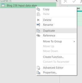
I call my new query Process_Sheet.
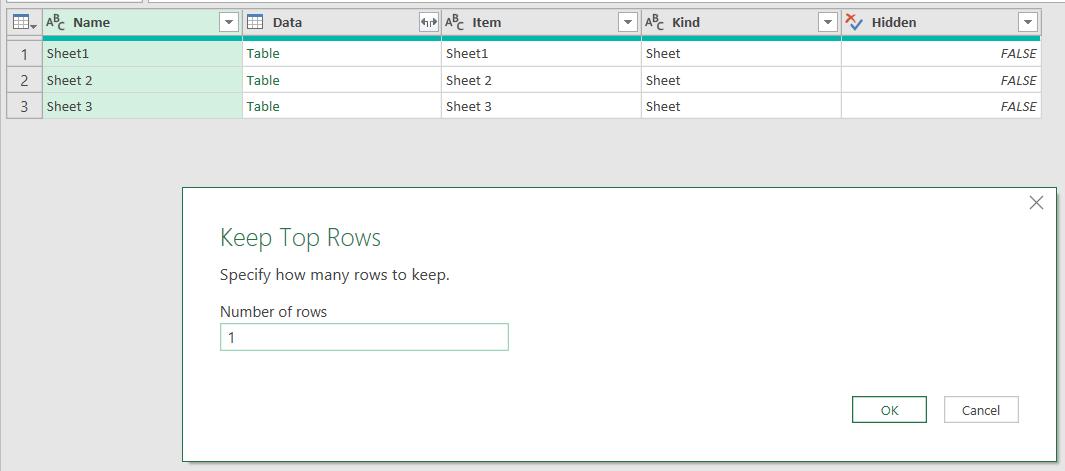
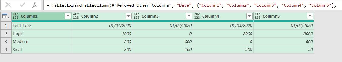
I filter to keep Sheet1, and select the Data column, which I right-click in order to remove the other columns. I can then expand it to see my data.
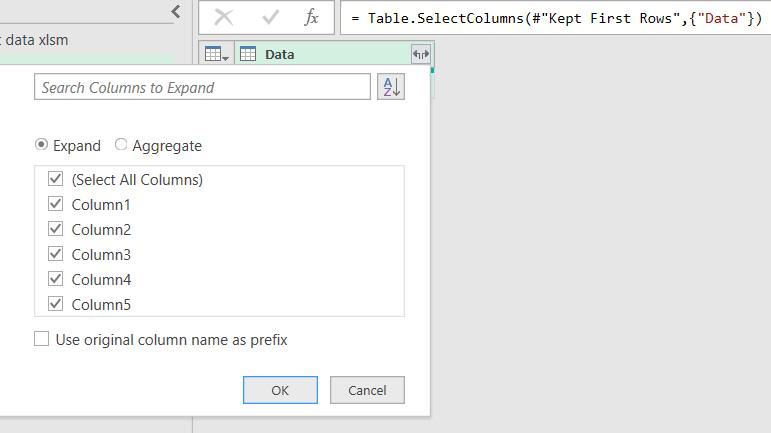
I don’t need a prefix.
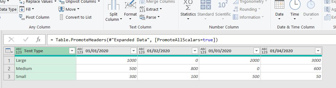
If I am going to append my data, I need the dates to be in a column. First, I promote my headers, which I can do in the Transform tab by ‘Using First Row as Headers’. If a ‘Change Type’ step is created, I must delete it, so that the column names are not referenced (as they will be different for the other sheets).
I can then select the Tent Type column and unpivot everything else.
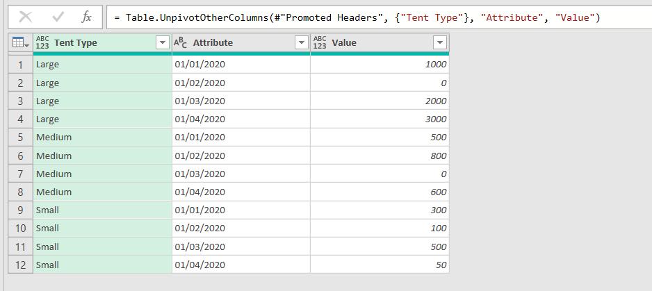
This looks good; I can now move onto the next step. This query is going to be a function, but first I need to set up a parameter, which will indicate which sheet is being processed. I can manage parameters on the Home tab.
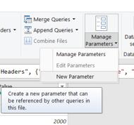
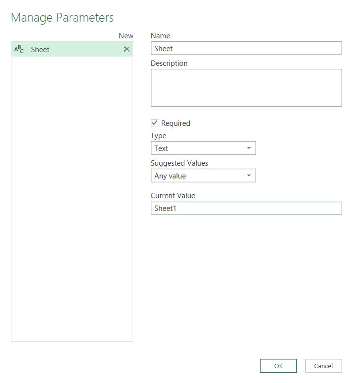
I create a new parameter, Sheet.
Sheet must be text, and it will be required by my new function. To begin with, Sheet will have a value of ‘Sheet1’.
Back in my Process_Sheet query, I go back to the ‘Filtered Rows’ step where I selected ‘Sheet1’. I am going to use the parameter instead.
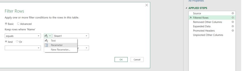
I choose my new parameter and click ‘OK’.
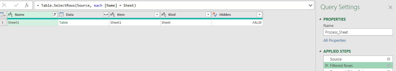
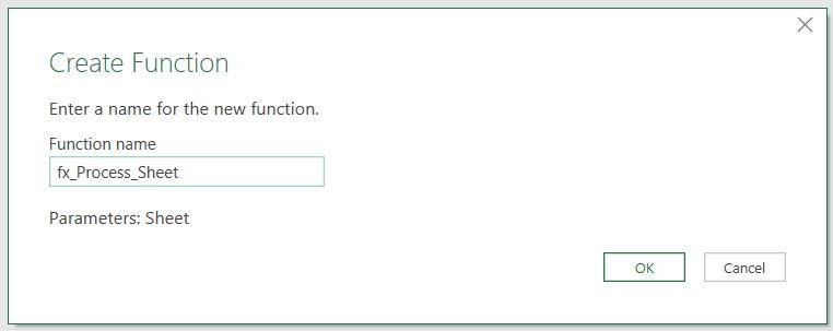
Because the default value is ‘Sheet1’, the parameter works in the same way as before. Now I need to make this query into a function.
I am prompted for a function name, which I call fx_Process_Sheet.
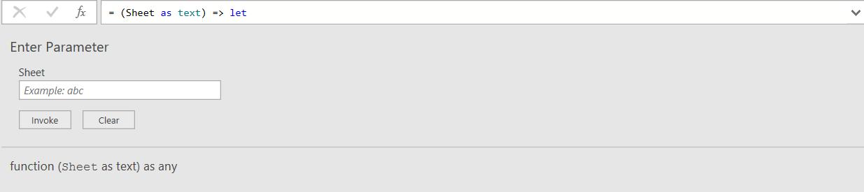
My function is ready to use.
Back in my original query, I want to invoke my function. In the ‘Add Column’ tab, I can ‘Invoke Custom Function’ and pass in the sheet name.
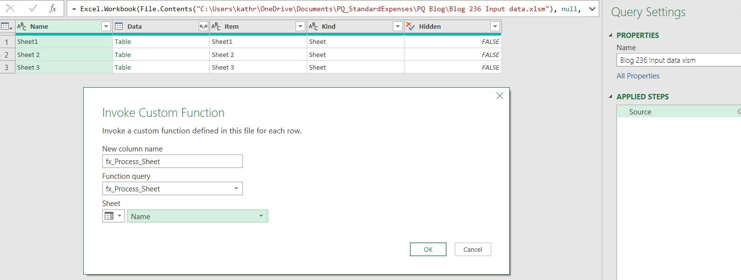
Clicking ‘OK’ gives me a new column. This should hold all the data I need.
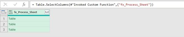
I can now expand it.
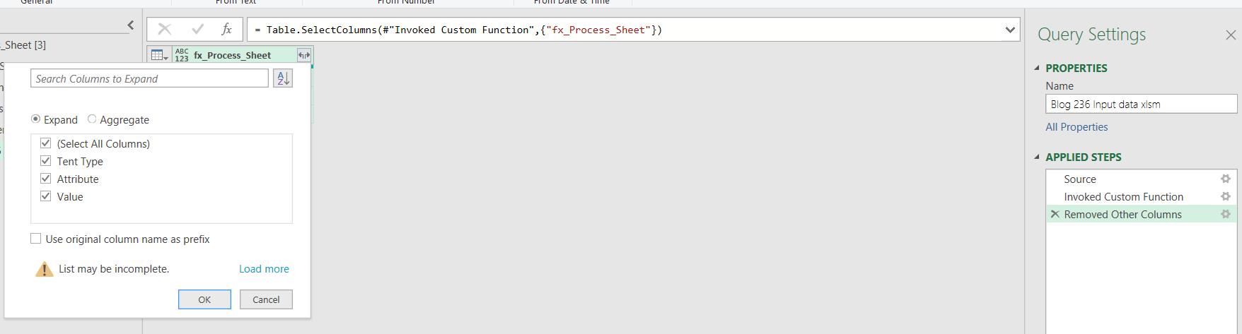
I select all columns and click ‘OK’.
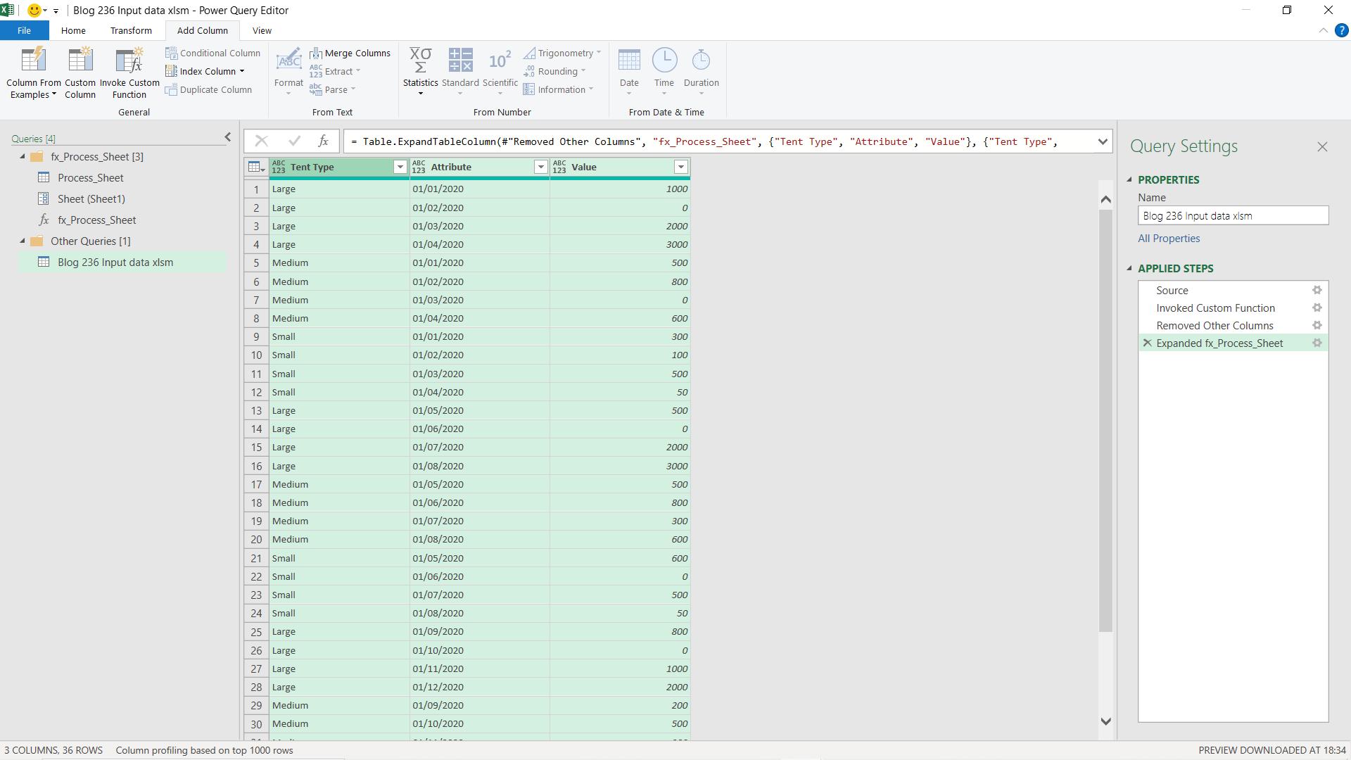
I have my data, I just need to change the data types on the Transform tab, rearrange it, and rename my columns.
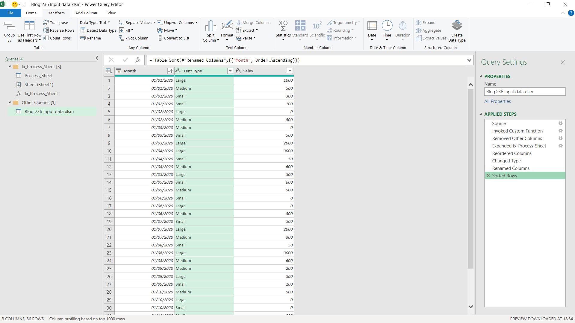
Come back next time for more ways to use Power Query!