A to Z of Excel Functions: The DVAR Function

Welcome back to our regular A to Z of Excel Functions blog.  Today we look at the DVAR function.

The DVAR function

This function estimates the variance of a population based on a sample by using the numbers in a field (column) of records in a list or database that match conditions that you specify.  The variance of a random variable X is the expected value (the average) of the squared deviation from the mean of the range of values of X, μ = E[X], i.e.

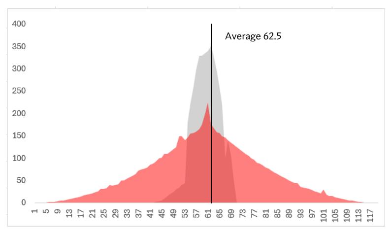
Two distributions with the same mean, but different variances.

Given that the standard deviation (σ) is given by:  

It is clear that the variance is the square of the standard deviation and hence is related accordingly with the DSTDEV function.

The DVAR function employs the following syntax to operate:

The DVAR function has the following arguments:

• database: this is required and represents the range of cells that makes up the list or database. A database is a list of related data in which rows of related information are records and columns of data are fields. The first row of the list contains labels for each column
• field: indicates which column is used in the function. Make sure you enter the column label enclosed between inverted commas (double quotation marks), e.g. "Age" or "Yield", or a number (without quotation marks) that represents the position of the column within the list, that is, 1 for the first column, 2 for the second column, and so on. Microsoft’s documentation states that this argument is required. We’re not convinced. If field is omitted, DVAR identifies the sum of all of the records in the table that match the criteria
• criteria: is the range of cells that contains the conditions you specify. You can use any range for the criteria argument, as long as it includes at least one column label and at least one cell below the column label in which you specify a condition for the column.

It should be further noted that:

• you can use any range for the criteria argument, as long as it includes at least one column label and at least one cell below the column label for specifying the condition, e.g. if the range G1:G2 contains the column label Income in G1 and the amount 10,000 in G2, you could define the range as MatchIncome and use that name as the criteria argument in the database functions (although do note that in the Excel web application, you cannot define named ranges yet)
• although the criteria range can be located anywhere on the worksheet, do not place the criteria range below the list. If you add more information to the list, the new information is added to the first row below the list. If the row below the list is not blank, Excel cannot add the new information
• make sure that the criteria range does not overlap the list
• to perform an operation on an entire column in a database, enter a blank line below the column labels in the criteria range.

Please see my example below:

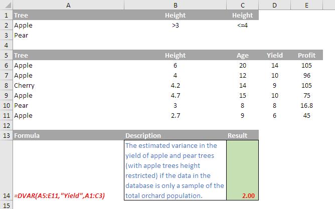
Criteria Examples

Typing an equal sign in a cell indicates you want to enter a formula.  To display text that includes an equal sign, surround the text and the equal sign with double quotes, like so:

"=Liam"

You also do that if you're entering an expression (a combination of formulas, operators, and text) and you want to display the equal sign instead of have Excel use it in a calculation. For example:

=''= entry '' 

Where entry is the text or value you want to find.  For example:

• When filtering text data, Excel does not distinguish between uppercase and lowercase characters. However, you can use a formula to perform a case-sensitive search (see below).

The following sections provide examples of complex criteria.

Multiple criteria in one column

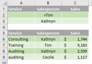
Boolean logic: (Salesperson = "Tim" OR Salesperson = "Kathryn")

To find rows that meet multiple criteria for one column, type the criteria directly below each other in separate rows of the criteria range.

e.g. In the following data range (A5:C9), the criteria range (B1:B3) displays the rows that contain either "Tim" or "Kathryn" in the Salesperson column (B5:B9).

Multiple criteria in multiple columns where all criteria must be true

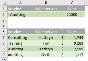
Boolean logic: (Service = "Auditing" AND Sales > 1500)

To find rows that meet multiple criteria in multiple columns, type all of the criteria in the same row of the criteria range.

In the following data range (A5:C9), the criteria range (A1:C2) displays all rows that contain "Auditing" in the Service column and a value greater than $1,500 in the Sales column (C5:C9).

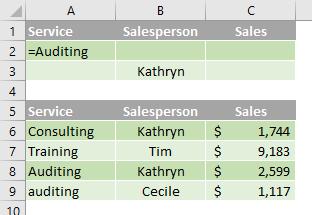
Multiple criteria in multiple columns where any criteria can be true

Boolean logic: (Service = "Auditing" OR Salesperson = "Kathryn")

To find rows that meet multiple criteria in multiple columns, where any criteria can be true, type the criteria in different rows of the criteria range.

In the following data range (A5:C9), the criteria range (A1:B3) displays all rows that contain "Auditing" in the Service column (C5:C9) or "Kathryn" in the Salesperson column (B5:B9).

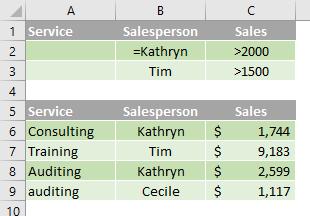
Multiple sets of criteria where each set includes criteria for multiple columns

Boolean logic: ( (Salesperson = "Kathryn" AND Sales >2000) OR (Salesperson = "Tim" AND Sales > 1500) )

To find rows that meet multiple sets of criteria, where each set includes criteria for multiple columns, type each set of criteria in separate rows.

In the following data range (A5:C9), the criteria range (B1:C3) displays the rows that contain both "Kathryn" in the Salesperson column and a value greater than $2,000 in the Sales column, or displays the rows that contain "Tim" in the Salesperson column (B5:B9) and a value greater than $1,500 in the Sales column (C5:C9).

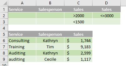
Multiple sets of criteria where each set includes criteria for one column

Boolean logic: ( (Sales > 2000 AND Sales <= 3000 ) OR (Sales < 1500) )

To find rows that meet multiple sets of criteria, where each set includes criteria for one column, include multiple columns with the same column heading.

In the following data range (A5:C9), the criteria range (C1:D3) displays rows that contain values between 2,000 and 3,000 and values less than 1,500 in the Sales column (C5:C9).

Criteria to find text values that share some characters but not others

To find text values that share some characters but not others, do one or more of the following:

• type one or more characters without an equal sign (=) to find rows with a text value in a column that begin with those characters. For example, if you type the text Lia as a criterion, Excel finds "Liam", "Liar" and "Lianne"
• use a wildcard character.

The following wildcard characters can be used as comparison criteria:

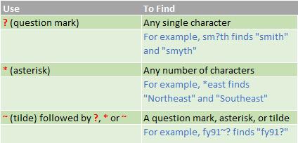
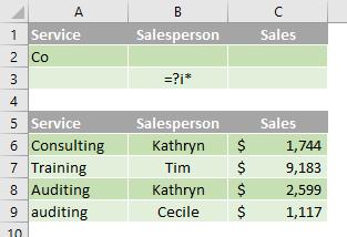
In the following data range (A5:C9), the criteria range (A1:B3) displays rows with "Co" as the first characters in the Service column or rows with the second character equal to "i" in the Salesperson column (B5:B9).

Criteria created as the result of a formula

You can use a calculated value that is the result of a formula as your criterion. Remember the following important points:

• the formula must evaluate to TRUE or FALSE
• because you are using a formula, enter the formula as you normally would, and do not type the expression in the following way:
  
  =''= entry ''
  
  
• do not use a column label for criteria labels; either keep the criteria labels blank or use a label that is not a column label in the range (in the examples below, Calculated Average and Exact Match)
• if you use a column label in the formula instead of a relative cell reference or a range name, Excel displays an error value such as #NAME? or #VALUE! in the cell that contains the criterion.  You can ignore this error because it does not affect how the range is filtered
• the formula that you use for criteria must use a relative reference to refer to the corresponding cell in the first row (in the examples below, C6 and A6)
• all other references in the formula must be absolute references.

The following subsections provide specific examples of criteria created as the result of a formula.

Filtering for values greater than the average of all values in the data range

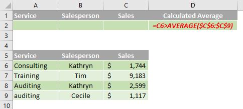
In the following data range (A5:C9), the criteria range (D1:D2) displays rows that have a value in the Sales column greater than the average of all the   values (C6:C9). In the formula, "C6" refers to the filtered column (C) of the first row of the data range (6).

Filtering for text by using a case-sensitive search 

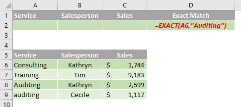
In the data range (A5:C9), the criteria range (D1:D2) displays rows that contain "Auditing" in the Service column by using the EXACT function to perform a case-sensitive search (A5:A9).  In the formula, "A6" refers to the filtered column (A) of the first row of the data range (6).

We’ll continue our A to Z of Excel Functions soon. Keep checking back – there’s a new blog post every business day.

A full page of the function articles can be found here.