
A to Z of Excel Functions: The GROUPBY Function
4 December 2023
Welcome back to our regular A to Z of Excel Functions blog. Today we look at the GROUPBY function.
The GROUPBY function
The GROUPBY function allows you to create a summary of your data formulaically. It supports grouping along one axis and aggregating the associated values. For instance, if you had a table of sales data, you might generate a summary of sales by year, or by salesperson, or by category, or by…
In essence, it allows you to group, aggregate, sort and filter data based upon the fields you specify.
The syntax of the GROUPBY function is given by:
GROUPBY(row_fields, values, function, [field_headers], [total_depth], [sort_order], [filter_array])
It has the following arguments:
- row_fields: this is required, and represents a column-oriented array or range that contains the values which are used to group rows and generate row headers. The array or range may contain multiple columns. If so, the output will have multiple row group levels
- values: this is also required, and denotes a column-oriented array or range of the data to aggregate. The array or range may contain multiple columns. If so, the output will have multiple aggregations
- function: also required, this is an explicit or eta reduced lambda (e.g. SUM, PERCENTOF, AVERAGE, COUNT) that is used
to aggregate values. A vector of
lambdas may be provided. If so, the
output will have multiple aggregations.
The orientation of the vector will determine whether they are laid out
row- or column-wise
- field_headers: this and the remaining arguments are all optional. This represents a number that specifies
whether the row_fields and values have headers and whether field
headers should be returned in the results.
The possible values are:
- Missing: Automatic
- 0: No
- 1: Yes and don't show
- 2: No but generate
- 3: Yes and show
- total_depth: this optional argument determines whether the row headers should
contain totals. The possible values are:
- Missing: Automatic, with grand totals and, where possible, subtotals
- 0: No Totals
- 1: Grand Totals
- 2: Grand and Subtotals
- -1: Grand Totals at Top
- -2: Grand and Subtotals at Top
- sort_order: again optional, this argument denotes a number indicating how rows
should be sorted. Numbers correspond
with the columns in row_fields followed by the columns in values. If the number is negative, the rows are
sorted in descending / reverse order. A
vector of numbers may be provided when sorting based upon only row_fields
- filter_array: the final optional argument, this represents a column-oriented one-dimensional array of Boolean values [1, 0] that indicate whether the corresponding row of data should be considered. It should be noted that the length of the array must match the length of row_fields.
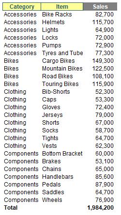
To show how GROUPBY works, consider the following Excel Table:

I have converted this data table into an Excel Table by selecting all the data and using Insert -> Table (CTRL + T) and calling the resultant Table tbl. Look, it’s late as I write this and I have no imagination, OK!?
I can summarise my Table very simply using the formula
=GROUPBY(tbl[Category],tbl[Sales],SUM)
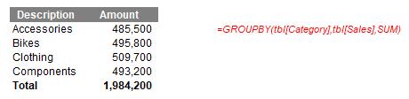
How easy is that!? Essentially, I am summing the sales (using the eta lambda SUM) by the Category field.
If you want to aggregate by more than one row_field, as stated above, this is possible. One way is to use HSTACK:
=GROUPBY(HSTACK(tbl[Year],tbl[Category]),tbl[Sales],SUM)
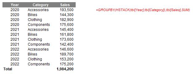
This simply combines the Year and Category fields in the tbl Table, and then sums Sales across them. However, I think I prefer the CHOOSECOLS approach:
=GROUPBY(CHOOSECOLS(tbl,1,2),tbl[Sales],SUM)
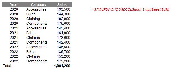
Here, the idea is that I shall SUM Sales by columns 1 (Year) and 2 (Category) of the tbl Table. This might not seem as clear as the HSTACK alternative at first glance as you have to refer to the Table to identify what the columns are. However, stick with me. Let me make the formula more complex:
=GROUPBY(CHOOSECOLS(tbl,MATCH(F$12,tbl[#Headers],0),
MATCH(G$12,tbl[#Headers],0)),tbl[Sales],SUM)
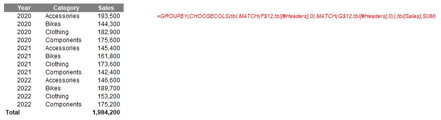
Looks horrible, yes? I have replaced the values 1 and 2 in the previous formula with
MATCH(F$12,tbl[#Headers],0)
and
MATCH(G$12,tbl[#Headers],0)
which return the positions in the Headers row of the Table tbl. Now, this may seem overkill but consider the following image:

Brilliant. I have changed the background colour of the first two headers to yellow. Well no, it’s a little more than that. I have used data validation dropdown lists (ALT + D + L) to create input headers!!

Thus, if I change the selections, I have dynamic summarisations, such as
or
Multiple summary statistics may be created similarly, or else you can simply connect them if the reporting fields are contiguous, e.g.
=GROUPBY(CHOOSECOLS(tbl,1,2),tbl[[Sales]:[Rating]],AVERAGE)
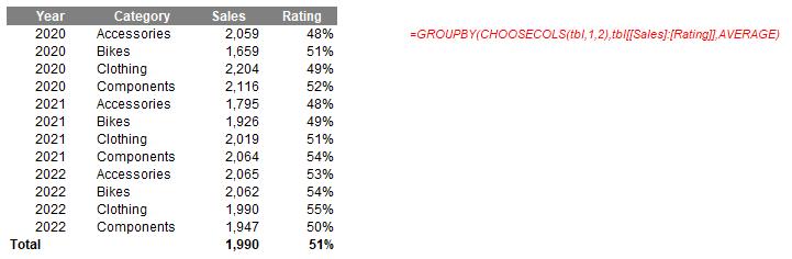
Here, tbl[[Sales]:[Rating]] may be used to specify the values as they are side by side.
Obviously, there are many more arguments to play with, but hopefully, you get the general idea, such as ranking the Item field in descending order by Sales using the formula
=GROUPBY(tbl[Item],tbl[Sales],SUM,,,-2)

Indeed, the outputs summarised don’t have to be numerical. A more comprehensive example summarising the Items field might look like this:
=GROUPBY(tbl[Category],tbl[Item],LAMBDA(x,ARRAYTOTEXT(SORT(UNIQUE(x)))))

We’ll continue our A to Z of Excel Functions soon. Keep checking back – there’s a new blog post every other business day.