A to Z of Excel Functions: The HSTACK Function

Welcome back to our regular A to Z of Excel Functions blog.  Today we look at the HSTACK function.

The HSTACK function

The HSTACK function returns the array formed by appending each of the array arguments in a column-wise fashion (Microsoft’s jargon, not ours).  It has the following syntax:  

The HSTACK function has the following argument(s):

• array: the first argument is required (others are optional) and represents the array(s) to append.

It should be noted that:

• HSTACK returns the array formed by appending each of the array arguments in a column-wise fashion.  The resulting arraywill be the following dimensions:
  • columns: the maximum of the column count from each of the array arguments
  • rows: the combined count of all the rows from each of the array arguments

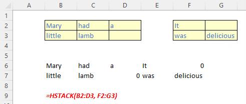
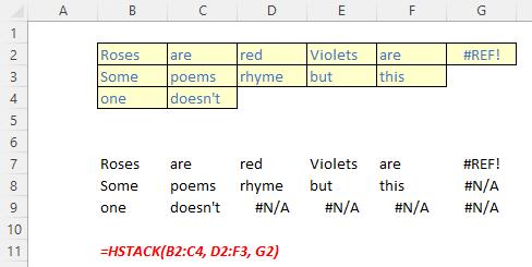
• Excel returns an #N/A error if an array has fewer rows or columns than the maximum in any selected array.  To remove the errors, you should use the IFERROR function.

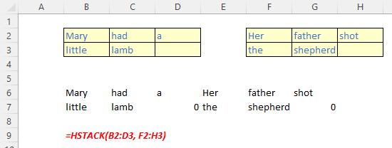
Please see my examples below: 

We’ll continue our A to Z of Excel Functions soon.  Keep checking back – there’s a new blog post every other business day.

A full page of the function articles can be found here.