A to Z of Excel Functions: The LOOKUP Function

Welcome back to our regular A to Z of Excel Functions blog. Today we look at the LOOKUP function.

The LOOKUP function

LOOKUP has two forms: an array form and a vector form. As a reminder:

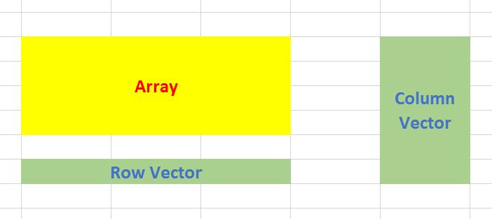
• An array is a collection of cells consisting of at least two rows and at least two columns
• A vector is a collection of cells across just one row (row vector) or down just one column (column vector).

The diagram should be self-explanatory:

The array form of LOOKUP looks in the first row or column of an array for the specified value and returns a value from the same position in the last row or column of the same array:

where:

• lookup_value is the value that LOOKUP searches for in an array.  The lookup_value argument can be a number, text, a logical value or a name or reference that refers to a value
• array is the range of cells that contains text, numbers, or logical values that you want to compare with lookup_value.

If array covers an area that is wider than it is tall (i.e. it has more columns than rows), LOOKUP searches for the value of lookup_value in the first row and returns the result from the last row.  Otherwise, LOOKUP searches for the value of lookup_value in the first column and returns the result from the last column instead.

The alternative form is the vector form:

The LOOKUP function vector form syntax has the following arguments:

• lookup_value is the value that LOOKUP searches for in the first vector
• lookup_vector is the range that contains only one row or one column
• result_vector is optional – if ignored, lookup_vector is used – this is the where the result will come from and must contain the same number of cells as the lookup_vector.

The lookup_value must be located in a range of strictly ascending values, i.e. where each value is larger than the one before and there are no duplicates.

LOOKUP is simple to use, doesn’t rely on row or index column numbers and allows modellers to create inputs that do not need to be specified for all periods modelled.  Let me demonstrate with the following example:

Imagine you have an annual model forecasting for many years into the future. Creating inputs will be time consuming if data has to be entered on a period by period basis. But there is a shortcut.

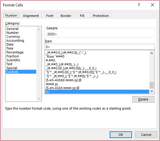
Do you see the data table in cells F12:K13 above? The value in the final cell of the first row is actually “2020” not “2020+”. It appears that way due to custom number formatting (CTRL + 1):

The syntax “0+” adds a plus sign to the number although Excel still reads the value as 2020. 

The formula uses the array version of LOOKUP, looking up the year in the first row of the data table and returning the corresponding value from the final row.  When a year is selected which is greater than 2020, the 2020 value is used as LOOKUP seeks out the largest value less than or equal to the value sought.  Therefore, we don’t need to have lengthy data tables – once we assume inputs will be constant thereafter, we can just curtail the input section.

Using the array form of LOOKUP is dangerous though.  What if someone accidentally inserts rows?  The lookup will “flip” to look the first and last columns instead, which is not what is required. Using the vector form is safer:

Whilst the formula contains one more argument, the formula is more stable.  Further, the lookup_vector and the result_vector do not need to be in the same worksheet or even the same workbook.  In fact, as long as there are the same number of elements in each, one can be a row vector and the other a column vector.

LOOKUP is very useful when the lookup_vector contains data in strict ascending order.  Where do we find this?  Dates in time series – LOOKUP is very useful for financial modelling / forecasting.  Just be careful though; consider the following scenario:

Here, the same formula generates an #N/A error.  This is because the date is smaller than the smallest value in the data range.  LOOKUP is not quite clever enough to use the first value unprompted, but a simple tweak of the formula will suffice:

Here, the formula has been modified to:

The added IF statement checks to see if the year is smaller than the first year in the data table and if so, returns the first result.  Simple.  It is with this final modification – in its vector form – that I usually use LOOKUP to return values for certain time periods where I do not want to have an input for each period modelled.  Very useful!

We’ll continue our A to Z of Excel Functions soon.  Keep checking back – there’s a new blog post every other business day.

 A full page of the function articles can be found here.