A to Z of Excel Functions: The MAP Function

Welcome back to our regular A to Z of Excel Functions blog. Today we look at the MAP function.

The MAP function

As one of the more recent Excel functions, MAP takes the honour of becoming Excel’s 500^th function – as agreed by fellow Excel Most Valuable Professional (MVP) Bill Jelen and ourselves.

You should be aware that Excel’s 500^th function (see earlier), the MAP function, does not actually return a map!

Instead, it returns an array formed by mapping each value in the array(s) to a new value and applying a LAMBDA to create a new value accordingly.  It has the following syntax:

where:

• array1: this is a required argument and represents the (first) array to be mapped
• array2 and subsequent arrays: these are optional arguments and represent additional arrays to be mapped
• lambda: this is a required argument which represents a LAMBDA which must be the final argument and must have a parameter for each array passed or another array to be mapped.

In short, MAP transforms values. 

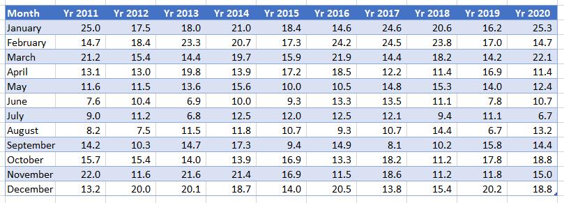
Let’s consider my Melbourne average temperatures data (in degrees Celsius):

If I want the year-on-year comparisons for each month where the average temperature is above 15 degrees Celsius, I can avoid using a “helper column” and instead use the formula

Here, the LAMBDA function returns values where the average temperature for the year is above 15 degrees Celsius, using the BYROW function, viz.

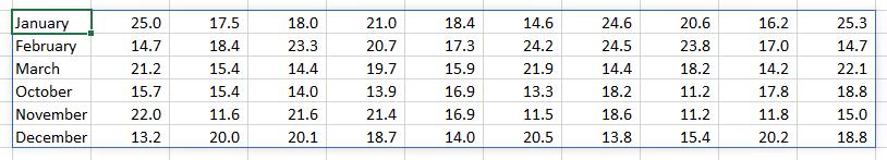
The problem is, these temperatures have all been provided in Celsius, which those of you in the United States (amongst other countries) may not understand.  If a US reader sees a temperature of 25 degrees, they will be breaking out the gloves, bobble hat and duffle coat, whereas us Aussies will be heading for the beach. 

We need to convert – transform – this data to Fahrenheit, so our US colleagues may better understand.  All I need to do is wrap the above formula in a MAP function:

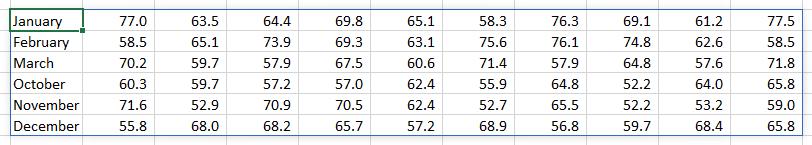
CONVERT(temperature, “C”, “F”) simply converts the variable temperature from degrees Celsius to degrees Fahrenheit. This is wrapped in an IF(ISNUMBER()) check to ensure that we don’t try to convert text values (as this would cause an error): the IF statement leaves the value of temperature “as is” in this instance, and LAMBDA just wraps around all of this in order to declare the variable temperature “work”, so that MAP may do its work.

It’s true you could generate this result in stages, but the whole idea of these LAMBDA helper functions is to be able to create dynamic arrays in one fell swoop.

We’ll continue our A to Z of Excel Functions soon. Keep checking back – there’s a new blog post every other business day.

A full page of the function articles can be found here.