A to Z of Excel Functions: The SIGN function

Welcome back to our regular A to Z of Excel Functions blog. Today we look at the SIGN function.

The SIGN function

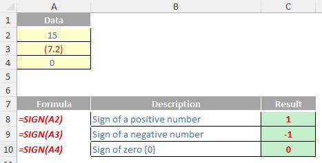
On the face of it, SIGN does not appear to be the most adventurous function in Excel.  It determines the sign of a number as:

• 1: if positive
• -1: if negative
• 0: if zero [0].

The SIGN function employs the following syntax to operate:

The SIGN function has the following argument:

• number: this is required and represents any real number.

The examples do not appear to enthral: 

Can we make this more exciting?  Yes we can!

Multiple Criteria with OR

Excel has two functions that deal with the logical operator OR:

1. OR(Condition_1,Condition_2,…) checks to see if any of the logical conditions specified are TRUE.  As long as at least one condition is TRUE, OR will be TRUE also
2. XOR(Condition_1,Condition_2,…) checks to see if each of the logical conditions specified are TRUE.  As long as at one and only one condition is TRUE, XOR will be TRUE also.  This is often referred to as “exclusive or”.

XOR is a new function in Excel 2013 and therefore is not backwards compatible with earlier versions.  In any case, OR and XOR do not work well with array formulae or functions that behave like arrays (“pseudo-array functions”), such as SUMPRODUCT.

At first glance, SUMPRODUCT(vector1,vector2,...) appears quite humble.  Consider the following sales report:

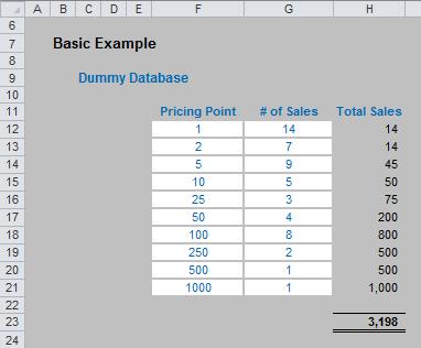
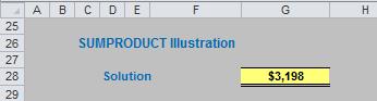
The sales in column H are simply the product of columns F and G, e.g.the formula in cell H12 is simply =F12*G12.  Then, to calculate the entire amount cell H23 sums column H.  This could all be performed much quicker using the following formula:

i.e. SUMPRODUCT does exactly what it says on the tin: it sums the individual products.    

Where SUMPRODUCT comes into its own is when dealing with multiple criteria.  This is done by considering the properties of TRUE and FALSE in Excel, namely:

TRUE*number = number (e.g. TRUE*7 = 7); and

FALSE*number = 0 (e.g. FALSE*7=0).

Consider the following example:

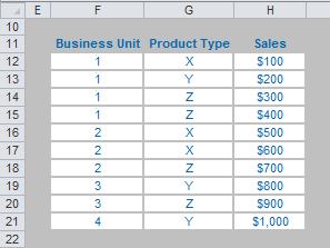
we can test columns F and G to check whether they equal our required values.  SUMPRODUCT could be used as follows to sum only sales made by Business Unit 1 for Product Z, viz.

For the purposes of this calculation, (F12:F21=1) replaces the contents of cells F12:F21 with either TRUE or FALSE depending on whether the value contained in each cell equals one [1] or not.  The brackets are required to force Excel to compute this first before cross-multiplying.

Similarly, (G12:G21=”Z”) replaces the contents of cells G12:G21 with either TRUE or FALSE depending on whether the value “Z” is contained in each cell. 

Therefore, the only time cells H12:H21 will be summed is when the corresponding cell in the arrays F12:F21 and G12:G21 are both TRUE, then you will get TRUE*TRUE*number, which equals the said number.

Notice that SUMPRODUCT is not an array formula (i.e. you do not use CTRL + SHIFT + ENTER), but it is an array function, so again it can use a lot of memory making the calculation speed of the file slow down.

But what if we only need one of these two criteria to be TRUE..?

Let us imagine we run a car sales company with four divisions: North, South, East and West.  Further, we only sell two types of car: the Mercudi and the Lexota:

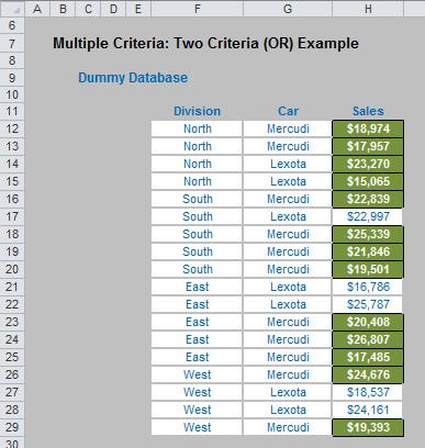
Imagine you are the General Manager responsible for the North Division and Mercudi sales.  Each month you have to provide a report summarising the total sales you are responsible for.  This requires analysis of multiple criteria, but it is an OR, rather than an AND, situation.

We need to include sales of North Division and sales of Mercudi.  However, if we do it this simply sales of Mercudi made by the North Division will be double counted:

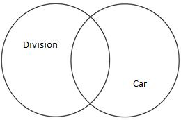
If we specify the criteria in the spreadsheet as follows:

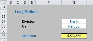
The formula in this instance would be:

However, there’s a simpler approach…

This is where  SIGN(number) comes in!  To recall:

• 1 if number is positive;
• 0 if number is zero; and
• -1 if number is negative.

It’s only when you start combining this function with SUMPRODUCT do you realise how useful it can be.  For example, in our scenario above, consider the following formula:

Inside the nested SIGN function, there are two criteria:

• Whether the Division is North (F12:F29=G34); and
• Whether the car sold is the Mercudi (G12:G29=G35).

Each criterion will either be TRUE (1) or FALSE (0), so the possible values inside the SIGN function are zero (neither criteria satisfied), one (only one criterion satisfied) or two (both criteria satisfied).  If neither criterion is true, SIGN will return a value of zero; if one or more criteria is true, SIGN will return a value of one and hence sum the relevant values in column H.  This is precisely what is required.

With more criteria considered, the simplicity of SUMPRODUCT(SIGN) becomes even more pronounced.

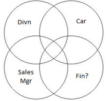
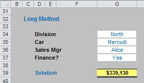
For the sake of brevity here, let’s jump straight to the four criteria scenario:

In this instance, having been a very successful General Manager, you have acquired greater responsibility: not only do you remain responsible for the North Division and Mercudi sales, but you are now mentor to salesperson Alice and for trying to push credit (finance) sales. 

As before, each month you have to provide a report summarising the total sales you are responsible for, which now considers four criteria: division, car, salesperson and finance:

If we specify the criteria in the spreadsheet as follows:

The “long” formula in this instance which would ensure the overlaps are not counted more than once would be:

It’s just so pretty.  PhDs are available for all those of you who can follow this formula in a heartbeat.  Why on earth would you use the SUMPRODUCT(SIGN) variant (below) instead? 

So yes, SIGN is useful in the world of modelling!

We’ll continue our A to Z of Excel Functions soon.  Keep checking back – there’s a new blog post every business day.

A full page of the function articles can be found here.