Charts and Dashboards: Dynamic Charts – Part 3

Welcome back to this week’s Charts and Dashboards blog series. We have been talking about creating Dynamic Tables using Tables and the OFFSET function. This week, let’s move on to Dynamic Named Ranges.

To recap, why do we need Dynamic Tables or Dynamic Range? The reason is whenever a list or data range is updated or modified, it is not certain that the report will be changed as per the data change. Dynamic Tables or Dynamic Range will help avoid this problem.

A Dynamic Range in Excel is a named range. An Excel Dynamic Named range is one of the more powerful techniques in Excel. Let’s look at the example below:

vs.

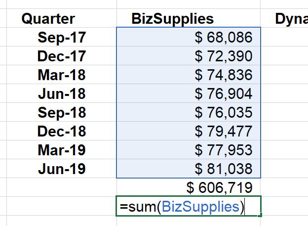
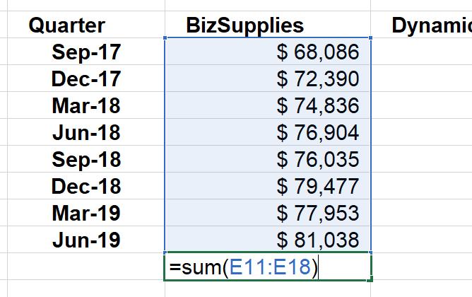
In the first figure’s summation, the range is from E11:E18, while in the second figure’s total, it is showing as BizSupplies. The reason is that the range B2:B10 has been named BizSupplies.

For a small set of data, it is not necessarily that a named range be applied. However, Dynamic Named Ranges make it much easier especially when you are working in larger set of data. Dynamic Named Ranges save us from going back to find and select targeted range of cells. Instead, we can just type the name which we have provided for that range.

Creating named ranges in Excel is straightforward.

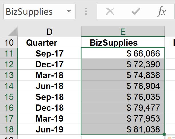
To do this, I can add a name for a range in the ‘Name Box’, after choosing the entire range that I want to name:

Alternatively, I may go to the Formulas tab on the Ribbon:

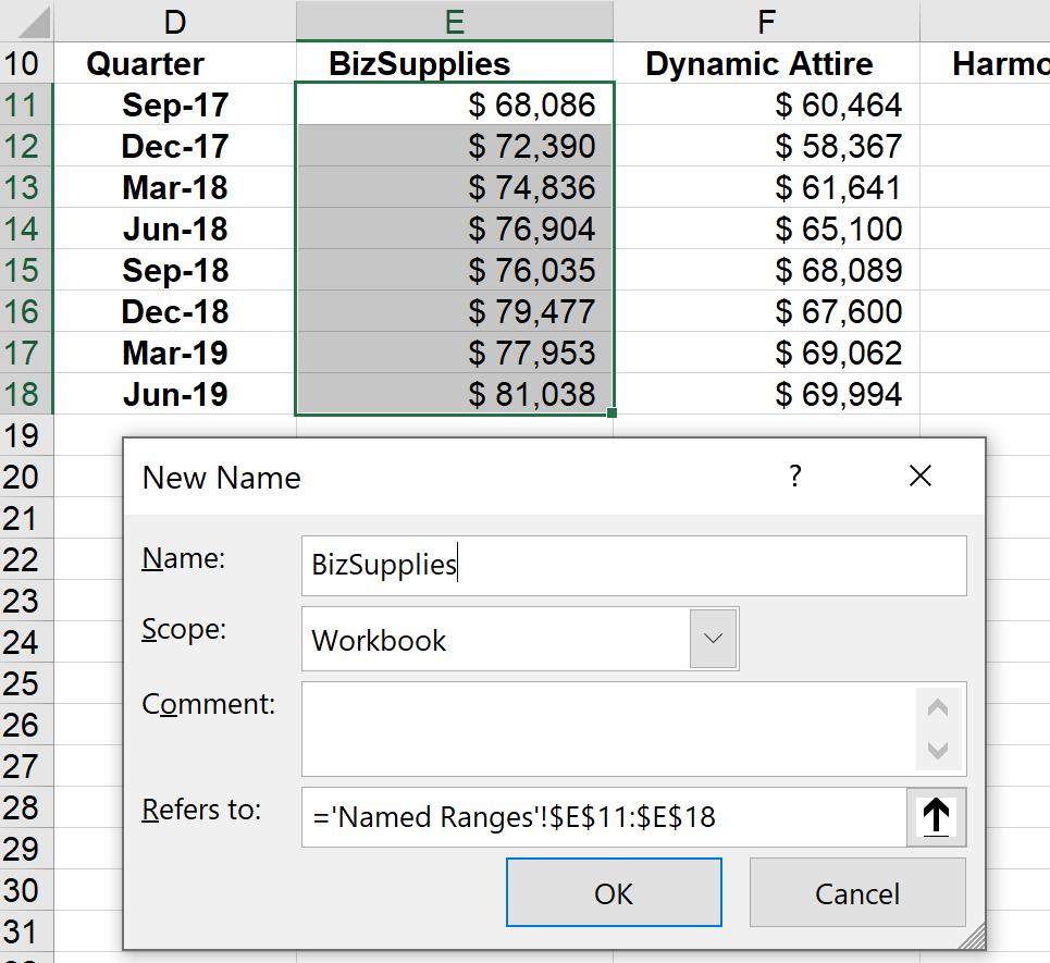
Then, the ‘New Name’ dialog will pop up, Here, I may fill in the ‘Name’, and select the range in the ‘Refers to’ field:

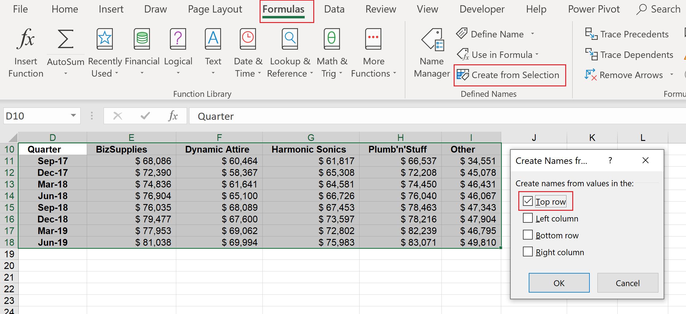
I can also create named ranges automatically when my data contains a large number of columns, by first choosing the whole data set, then click Formulas –> Name Manager –> Create from Selection. The ‘Create Names from Selection’ dialog will appear, where I may choose ‘Top row’ as the column name to use as the name for the range:

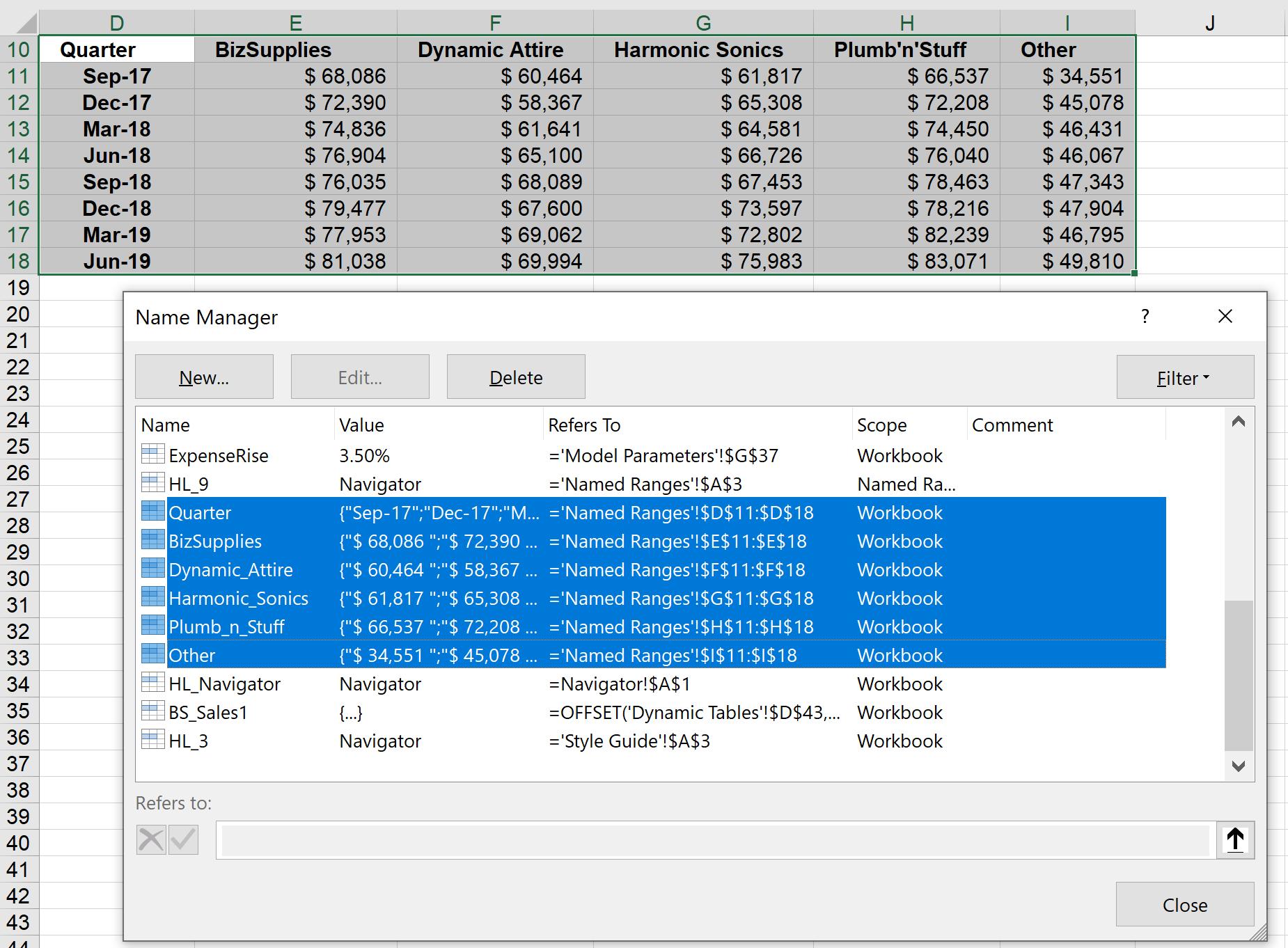
After that, when I choose the Formulas –> Name Manager, the list of names should be displayed:

This is just the first step. In a simple named range, it will take only the pre-determined range. In the case of data expansion, it will not expand dynamically. Therefore, we need to create a Dynamic Range in Excel. When we define an Excel Dynamic Named Range, as new items are added, the range will automatically expand.

To create this, let’s apply data validation to the named range that has already been set, navigating to the Data tab on the Ribbon and choosing ‘Data Validation’:

Change the 'Validation criteria' as the below dialog:

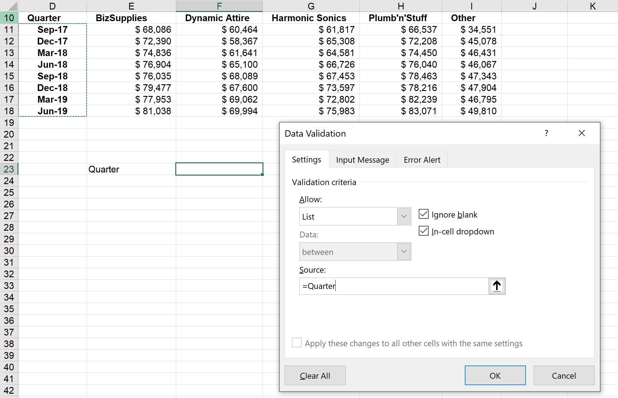
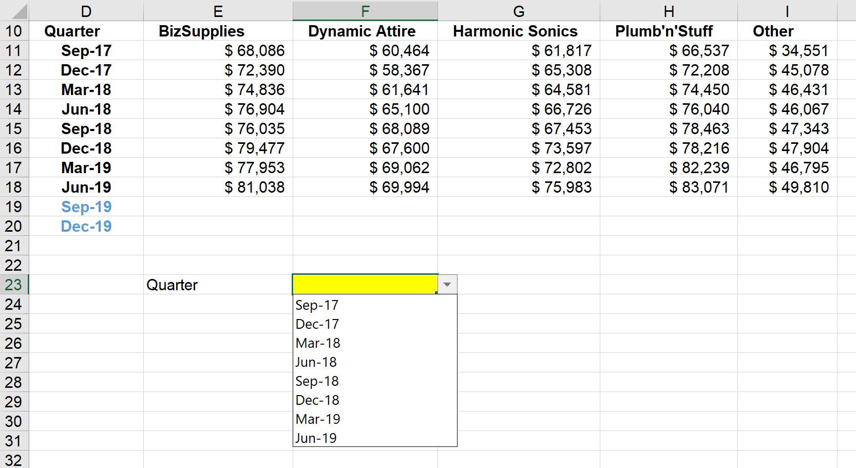
Now that the ‘Data Validation’ dialog for Quarter has been created, it displays all of the range in the Quarter column:

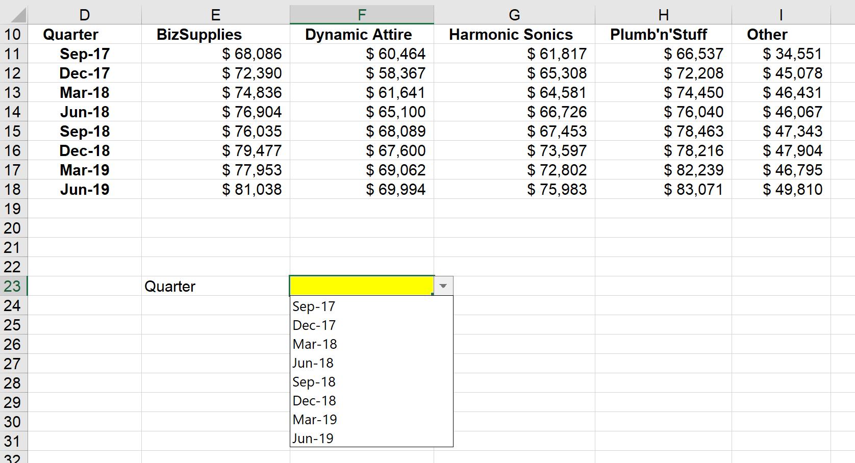
However, if I add more values to the column, these newly added values will not appear in the dropdown cell. This is because the range is not dynamic.

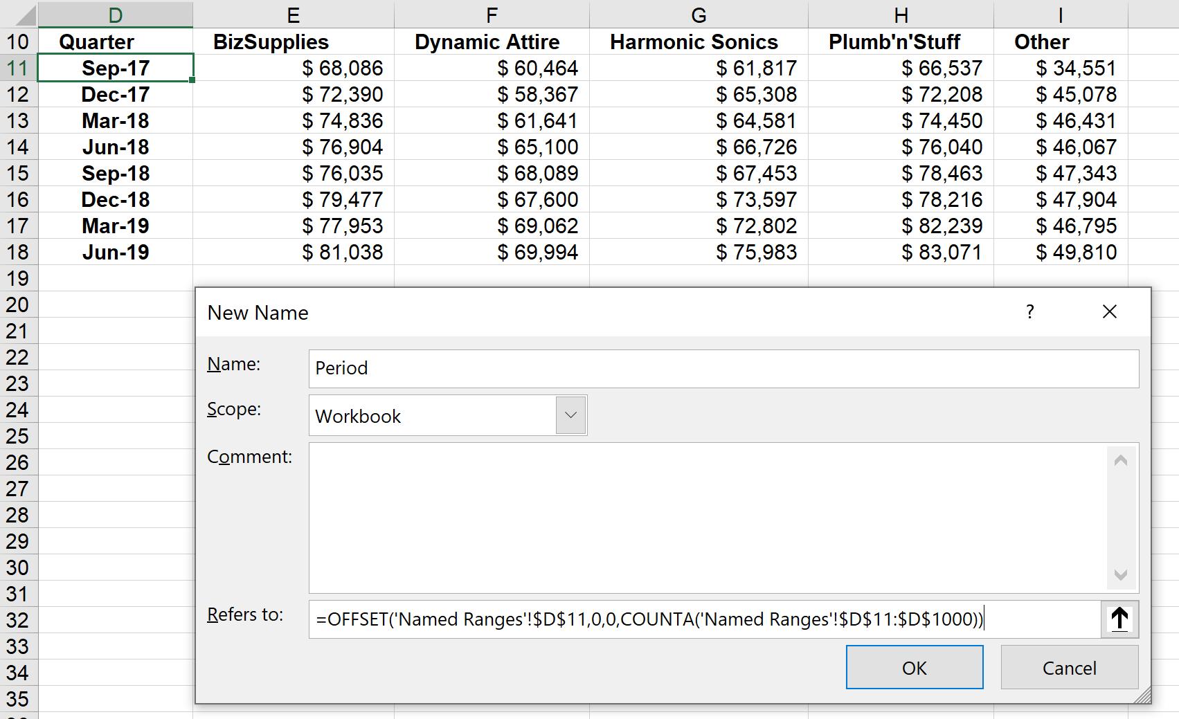
To fix and compare this, I create a new named range called Period, now using the OFFSET function as below, similar to the example provided with Dynamic Tables, so that newly added values will be counted:

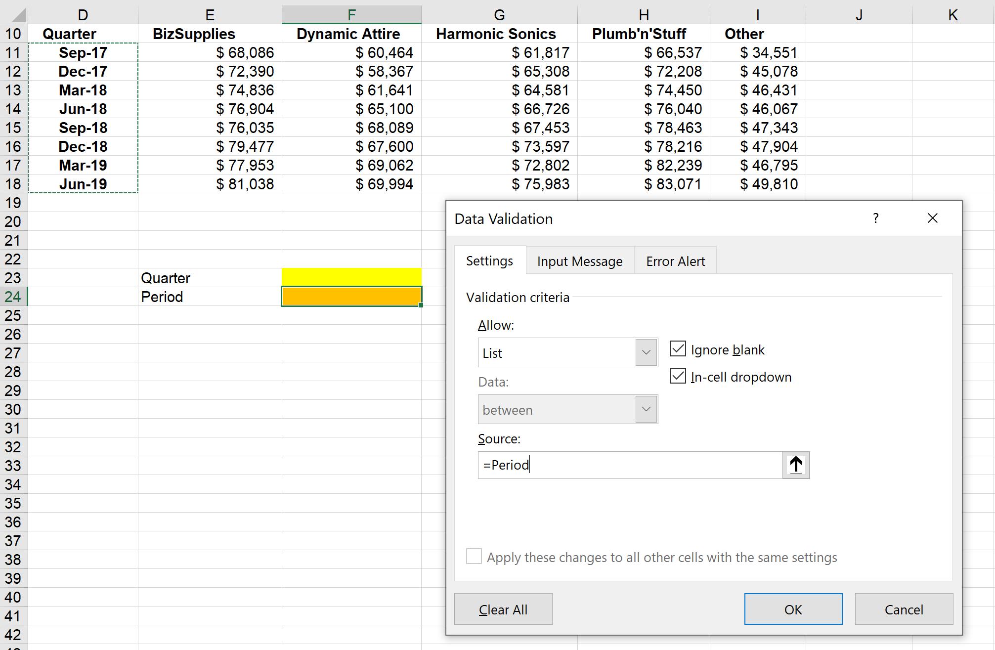
Then, I call the ‘Data Validation’ dialog. This time, the ‘Source’ will be the named range which has just been created using the OFFSET function, i.e. Period:

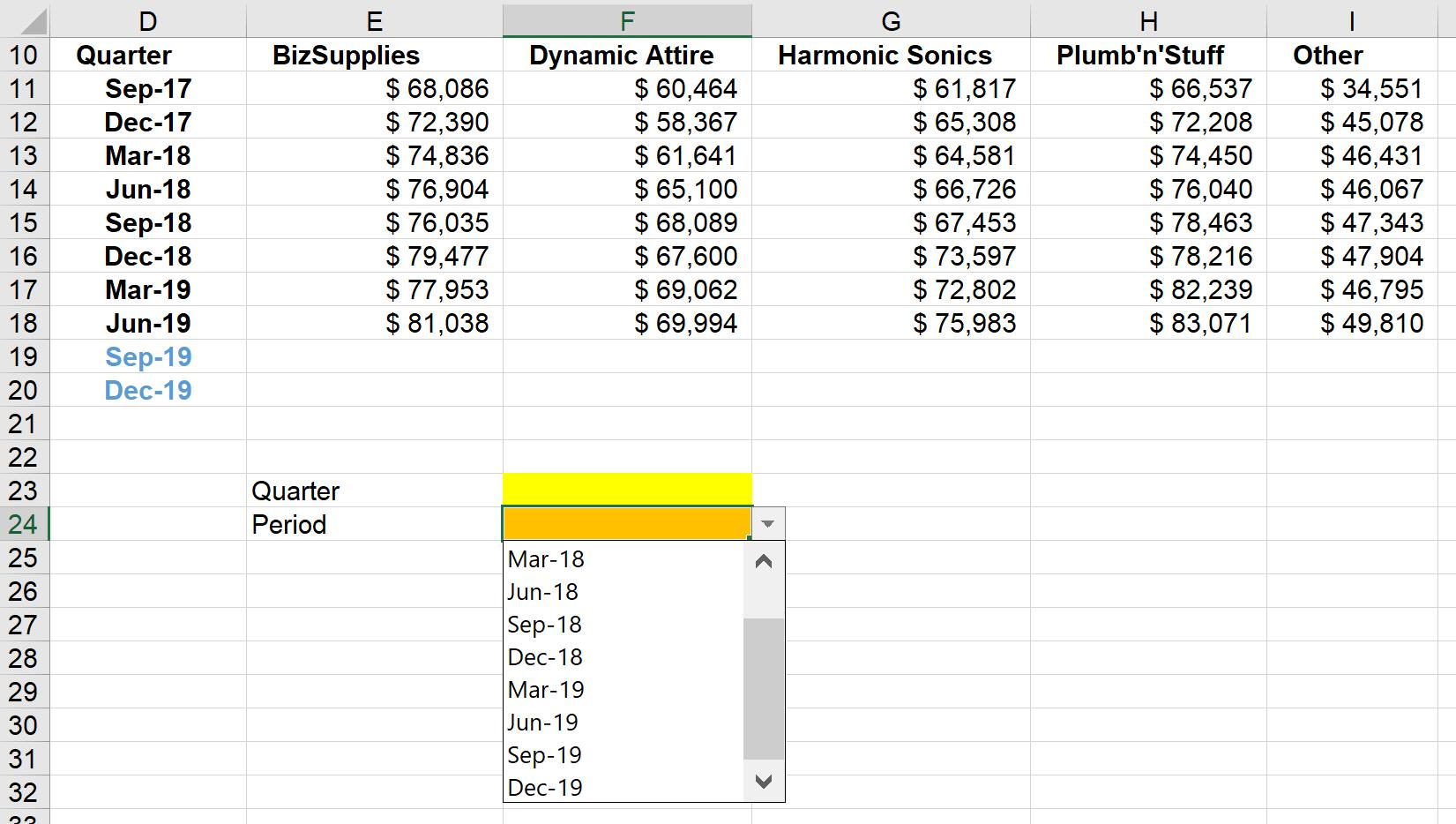
Here, I add values to the Quarter column. As new reports appear, I check that in the Period validation, new values are now displayed:

That’s it for this week, check back next week for more Charts and Dashboards tips.