
Monday Morning Mulling: May 2022 Challenge
30 May 2022
On the final Friday of each month, we set an Excel / Power Pivot / Power Query / Power BI problem for you to puzzle over for the weekend. On the Monday, we publish a solution. If you think there is an alternative answer, feel free to email us. We’ll feel free to ignore you.
The challenge this month was to create a PivotTable that showed the sales amount made by each salesperson in their individual business units, as well as a percentage breakdown for each business unit and the percentage contribution of each business unit to total sales. Easy, yes?
The Challenge
In this challenge, we required you to create a PivotTable that showed the amount of sales made by each salesperson in their individual business units, as well as a percentage breakdown for each business unit and the percentage contribution of each business unit to total sales.
You can download the question file here.
As always, there were a few requirements:
- this problem should be solved entirely in Power Pivot and with the help of measures
- filtering should not modify the proportion contribution of each business unit to total sales.
Suggested Solution
You can find our Excel file here which demonstrates our suggested solution. However, before explaining our solution, we will clarify the common idea how we came up with it first.
For Excel Office 365, Excel on the Web, and Office Beta / Insider versions
These Excel versions allow us to use DAX functions in Power Pivot which help shorten a lot of steps.
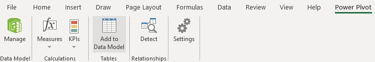
Firstly, we must begin by adding the data table to the Data Model in Power Pivot, so that we may manipulate it with DAX.
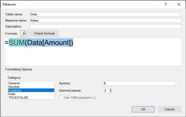
Secondly, create a new measure in Power Pivot for total sales using formula:
=SUM(Data(Amount))
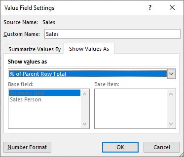
Note: Before moving on to the next step, I wish to point out that we may make a PivotTable like this by just changing the value field setting of the sales measure we defined above to ‘% of Parent Row Total’. This approach will breach our second condition since, in this circumstance, if you filter by business unit, the percentage breakdown will vary.
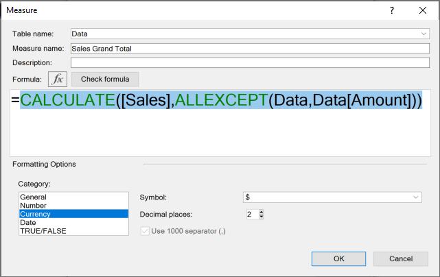
Thirdly, create a measure (Sales Grand Total) in Power Pivot for sales grand total using CALCULATE and ALLEXCEPT DAX functions. We are using ALLEXCEPT to remove all filters from grand total apart from the Data[Amount] column:
=CALCULATE([Sales], ALLEXCEPT(Data, Data[Amount]))
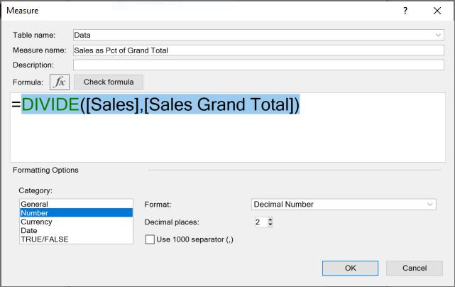
The next step would be to create a measure in Power Pivot for Sales as % of Grand Total by DIVIDE DAX function:
=DIVIDE([Sales], [Sales Grand Total])
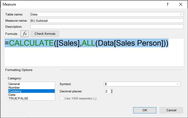
Then, we have to create a measure in Power Pivot for Business Unit Subtotal using CALCULATE and ALL DAX function:
=CALCULATE([Sales], ALL(Data[Sales Person]))
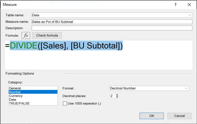
The next step would be to create a measure in Power Pivot for Sales as % of BU subtotal using:
=DIVIDE([Sales], [BU Subtotal])
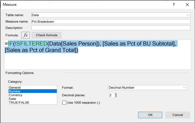
Moving on, we must create a measure in Power Pivot for ‘Pct Breakdown’ using IF and the ISFILTERED DAX functions:
=IF(ISFILTERED(Data[Sales Person]), [Sales as Pct of BU Subtotal], [Sales as Pct of Grand Total])
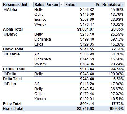
Finally, in the Insert section, we can insert a PivotTable from the Data Model. The PivotTable may then be added using ‘Business Unit’ and ‘Sales Person’ as row fields, and Sales and Pct Breakdown as value fields, viz.
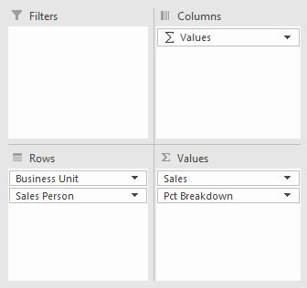
This will produce the result required:
The Final Friday Fix will return on Friday 24 June 2022 with a new Excel Challenge. In the meantime, please look out for the Daily Excel Tip on our home page and watch out for a new blog every business working day.