Monday Morning Mulling: October 2021 Challenge

On the final Friday of each month, we set an Excel / Power Pivot / Power Query / Power BI problem for you to puzzle over for the weekend.  On the Monday, we publish a solution.  If you think there is an alternative answer, feel free to email us.  We’ll feel free to ignore you.

This month, we just wanted you to convert numbers stored as Text into Numbers.  Easy, yes?

The Challenge

Sometimes, you may need to deal with numbers in the text format.  As you may know, there are various ways to convert them into “real” numbers.  This challenge is a little trickier, but you may come across it some day when using Excel.

One of our clients recently came up with this challenge.  They provided us with a list of numbers copied from their management information system into Excel.  It was in a text format that needed to be converted into numbers.

We have made up a similar list for this challenge that you can download here.

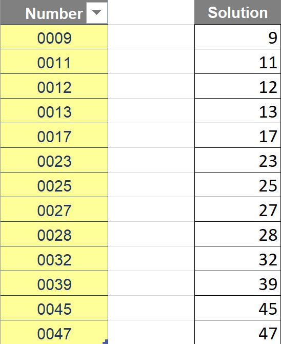
This month’s challenge was to write a formula that could be copied down to convert the list of numbers from text format into a numerical data type, like the ones on the right that you can see below:

There were some constraints:

• there should be no “helper” column
• this was a formula challenge: no Power Query / Get & Transform, Text to Columns or Flash Fill!
• the formula needed to be dynamic enough so that if we change from four digits to a different length, the formula must still work.

Suggested Solutions

You can find our Excel file here which demonstrates our two suggested solutions.

As you may know, to clean and convert Text to Number, there are several common ways to apply such as:

• functions (e.g. TRIM, CLEAN, N and VALUE)
• coercing techniques (e.g. using *1, +0 or -- in your formula)
• Paste Special, multiplying by one [1] or adding zero [0]
• Text to Columns
• Flash Fill
• etc.

However, after we had tried all the options above, we realised that they could not convert properly and / or did not meet the requirements of the question.

Before explaining our solutions, we will clarify how we came up with them first.

Brainstorming

After using some common ways as mentioned above, we tried to find out what kind of characters in the strings that did not allow us to convert Text to Numbers properly.

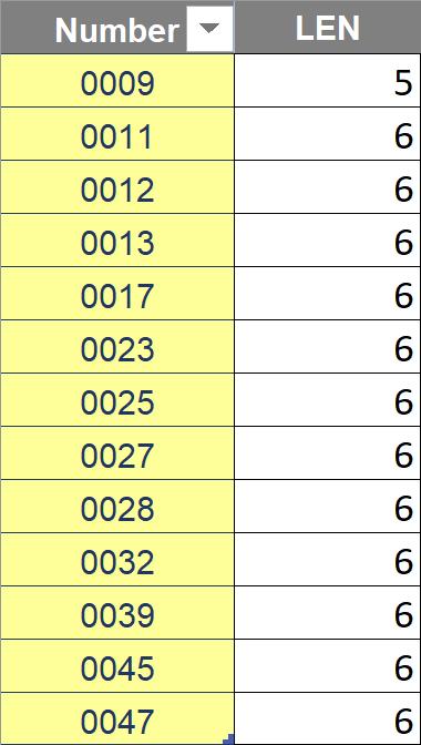
Firstly, we used LEN(text) function which returns number of characters in a text string.  According to the result below, all strings have more than four characters.  Hence, there must be other characters beside the four digit numbers that we could not see.

Secondly, we wanted to identify the positions of those unwanted characters.  Therefore, we split each character of the text strings into different cells by using a combination of MID, SEQUENCE and LEN functions.

While you may be familiar with MID and LEN functions, SEQUENCE is one of the Dynamic Arrays that are only available in Excel for Microsoft 365 / online versions.  You can read more on this in a blog we have written before.

The formula is as follows:

In the formula above:

• Numbers is the name of the table in the question.  Therefore, Numbers[@Number] specifies one row of column Number, where the above formula is located.
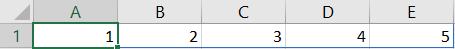
• SEQUENCE(1,LEN(Numbers[@Number])) will help us create a horizontal list of consecutive numbers from 1 to the last number which is equal to the length of the string. For example:

• The MID function will then extract each character of a string with the starting point one by one, equal to the number list created by SEQUENCE above.

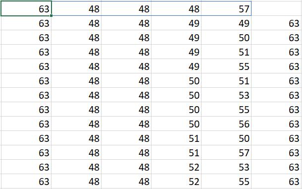
After you copy down the formula, the result should look like this:

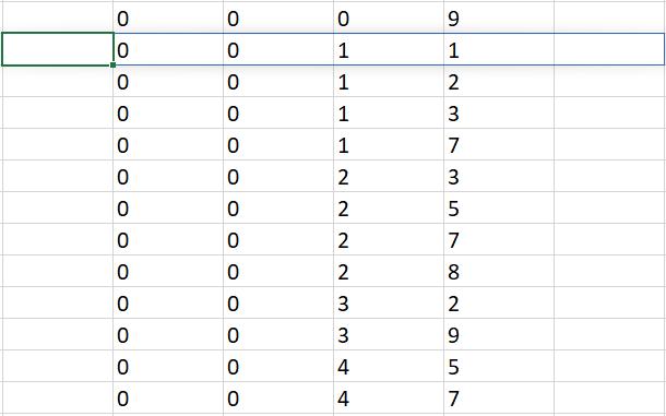
We can see that there are invisible characters at the beginning and the end of the strings.

Thirdly, we needed to identify what those invisible characters were.  We tried applying CODE and CHAR functions to our dynamic arrays above first.  CODE allows us to return a numeric code for the first character in a text string.  CHAR translates that code back into a character.

The result is as follows: the code of these “invisible” characters is apparently 63, viz.

However, when we used CHAR function to return a character, it returned a question mark (?). It seemed to be incorrect as “?” is still visible. Something was not right!

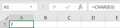
We realised that CODE and CHAR can only work with characters with number codes between 1 and 255.  Any codes above 255 cannot be identified so Excel returns a question mark (?).  Great.  Sorry, I meant “grate”.

Then, we used UNICODE and UNICHAR instead which have similar usages, but support higher number of characters.  The result is as follows:

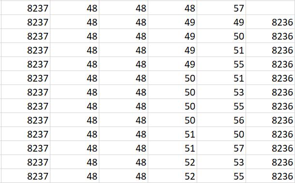
As you can see above, characters 63 have turned into “Left-To-Right Override” (8237) and “Pop Directional Formatting” (8236) which are both non-printable characters.  The rest is still the same.

The mystery was SOLVED!

In summary, we need to eliminate characters 8237 and 8236 before converting the text strings to numbers.

Returning to the Suggested Solution

The main function in our solutions is SUBSTITUTE.  This function has already been mentioned in our August 2021 Challenge.  It will be used to remove characters 8237 and 8236 from the text strings.  Thus, in order to specify the two characters 8237 and 8236 in the formula, we have two options:

Option 1: If you use Excel 2013 onwards, you can use the UNICHAR function to return the characters from their codes (i.e. 8237 and 8236).  The formula is as below:

Therefore, we use two SUBSTITUTE functions and two UNICHAR functions to replace those unwanted characters with blank, "".  Then, we add zero [+0] to force the remaining strings to become numbers.

Option 2: This option is for all current Excel versions.  Please note that as characters 8237 and 8236 are non-printable characters, you will not see them in the formula below.  Please copy the formula (not typing it again).

See you next month!

The Final Friday Fix will return on Friday 26 November 2021 with a new Excel Challenge.  In the meantime, please look out for the Daily Excel Tip on our home page and watch out for a new blog every business working day.