
Monday Morning Mulling: July 2023 Challenge
31 July 2023
On the final Friday of each month, we set an Excel / Power Pivot / Power Query / Power BI problem for you to puzzle over for the weekend. On the Monday, we publish a solution. If you think there is an alternative answer, feel free to email us. We’ll feel free to ignore you.
The Challenge
Imagine that you need to filter rows in a table that have specific keywords within the text strings contained therein. Manually filtering every single keyword and copying / pasting them to a new location can be a tedious and time-consuming process. To address this, we challenged you to develop a user-friendly solution that allows users to select the desired keywords and return a list having all the text strings associated with those keywords. You can download the original question file here.
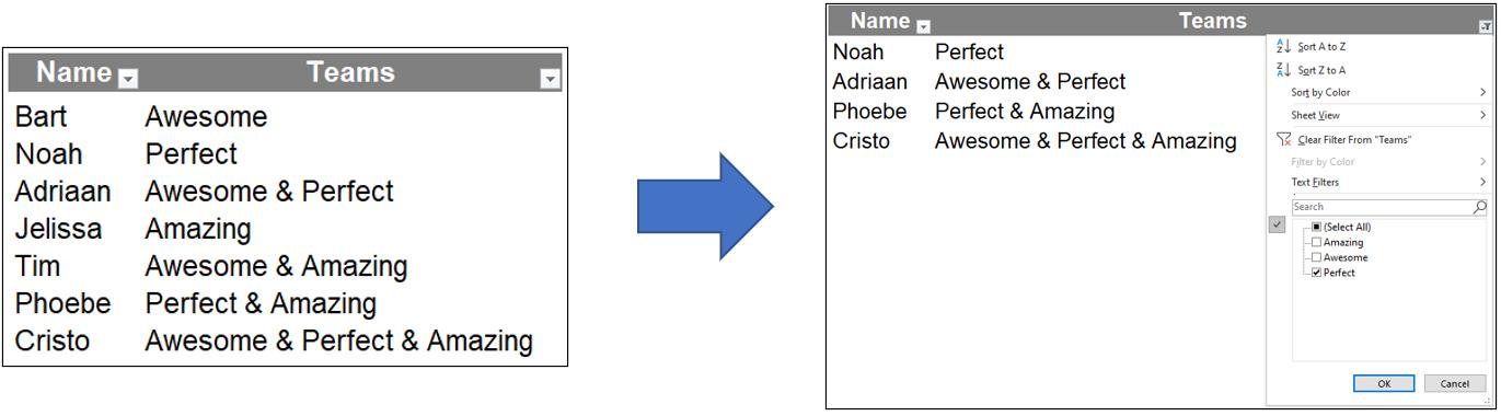
Your aim was to create a filter using the keywords "Awesome", "Amazing", and "Perfect" as filter criteria, as shown in the picture below:
As always, there were some requirements:
- no Power Query / Get & Transform or VBA was allowed
- the formula(e) should be dynamic so that they should update when a new entry was added.
Suggested Solution 1
You can find our Excel file here, which shows our suggested solution. The steps are detailed below.
Find the keywords
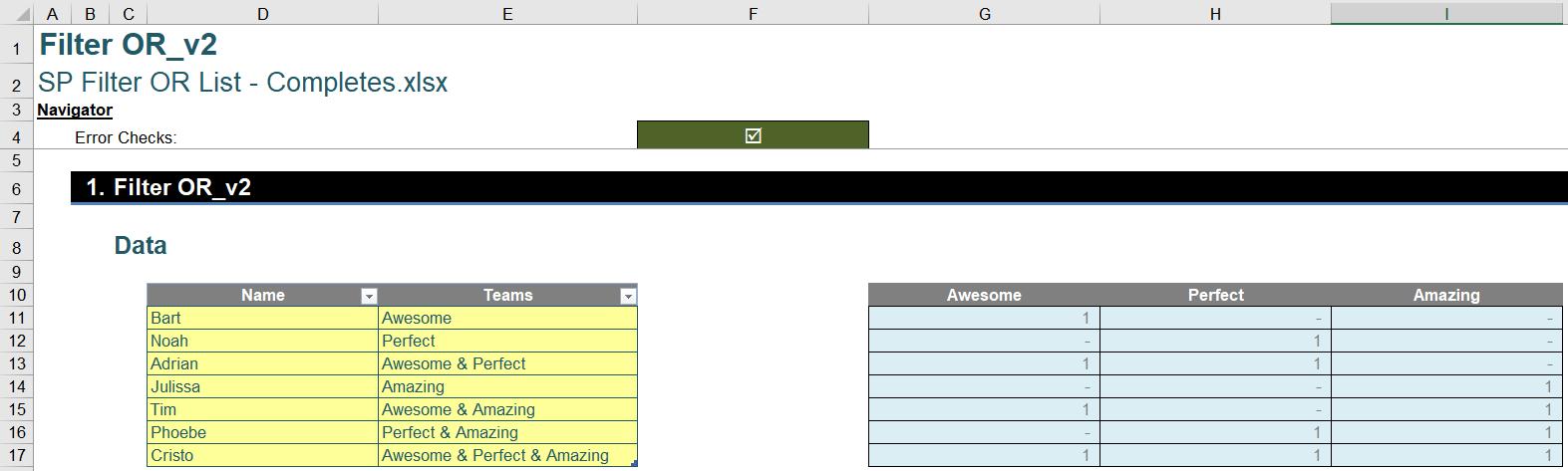
To begin, we create four [4] new columns in the Data_v1 table. One is named Included and the other three [3] represent the heading names based upon the keywords provided:
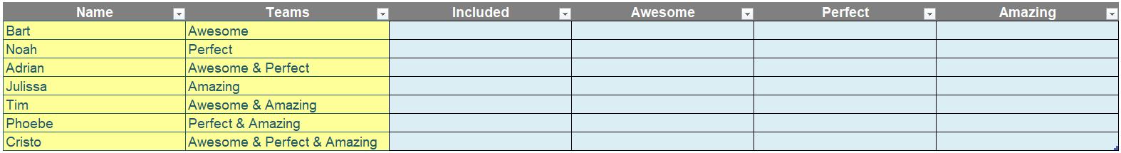
We accept this is a manual interaction as Table headers may not contain formulae.
To check whether the text strings in the Data_v1[Teams] column have specific keywords, we need to create a formula that uses the ISNUMBER and SEARCH functions. These functions work together to confirm the keywords are within the text strings (note that the FIND function could also be used, but beware that it's case-sensitive and requires an exact match between the capitalisation of the keywords and text strings).
=ISNUMBER(SEARCH(Data_v1[[#Headers],[Awesome]],[@Teams]))*1
The SEARCH function will return a number if the keywords is found within the text string. If the text string did not contain the keyword, then it will return #VALUE! Then, the ISNUMBER checks whether the output of the SEARCH function is a number or not and will return TRUE or FALSE accordingly.
At this point, we can choose to keep it as logical value or turn it into number. We will change all these logical values into numbers, so we multiply the numbers by one [1]. Therefore, all TRUE values will be restated as one [1] and all FALSE values will turn to zero [0]. Similarly, we will do the same for the other two [2] columns, viz.
=ISNUMBER(SEARCH(Data_v1[[#Headers],[Perfect]],[@Teams]))*1
=ISNUMBER(SEARCH(Data_v1[[#Headers],[Amazing]],[@Teams]))*1
Hidden power of SUBTOTAL
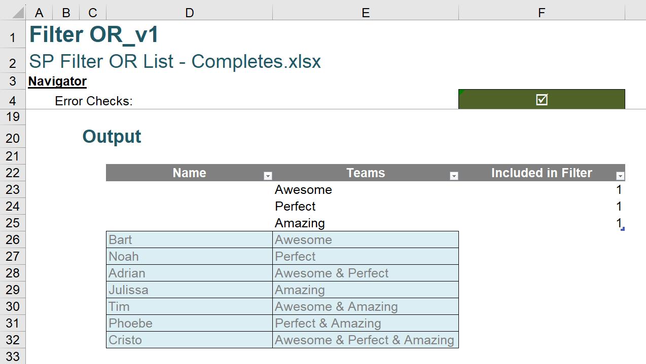
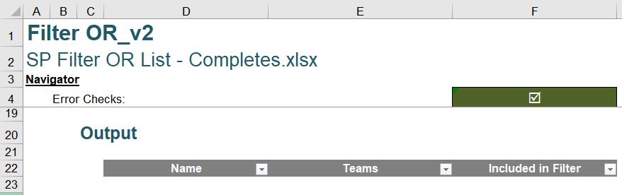
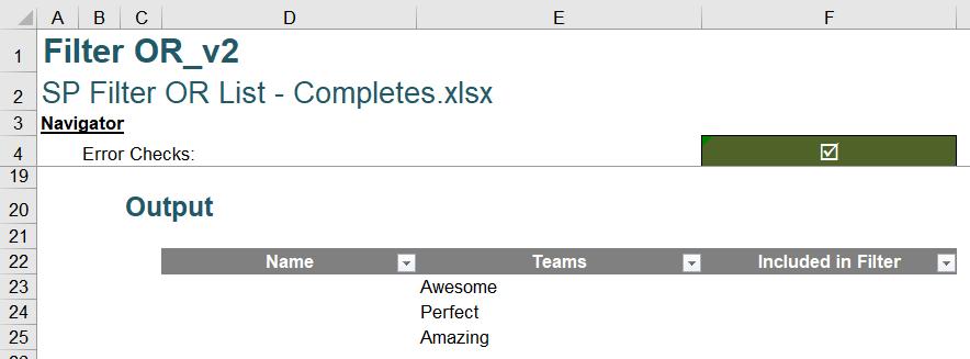
Let’s move on the Output table. In this table, we first enter the keywords of this challenge in the Teams column and we will leave the Name column blank:
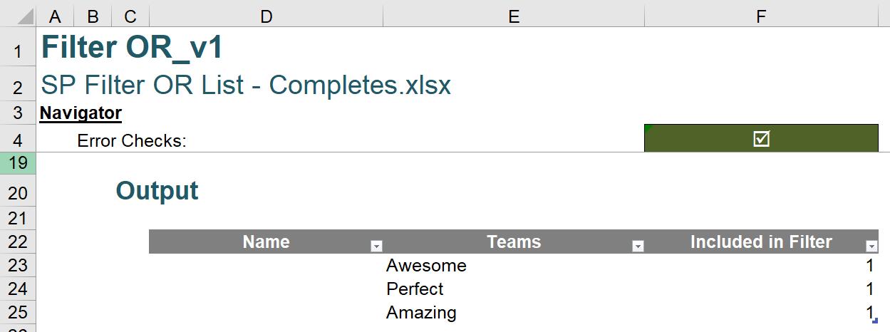
Then, we added one column to this Table and we call this column ‘Included in Filter’. This column will specify which keywords to include in the filter. The formula for this new column will be:
=SUBTOTAL(103,[@Teams])
The SUBTOTAL function has the advantage of being able to exclude hidden cells from calculations. When the function_num is greater than 100, the SUBTOTAL function will not include any hidden cells in the calculation.
Using function_num 103 of SUBTOTAL, which is COUNTA, will return one [1] if a cell is not hidden and zero [0] if the cell is hidden. For instance, if we completely hide the row 23, the result will be as follows:
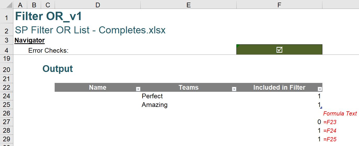
As we can see cell F23 has a value of zero [0] while another unhidden cell has a value of one [1].
We did not format this table or add any colouring as we will need to set the pixel height of these rows to one [1] later, so not putting formatting here will prevent any colours condensing together later on.
Matching keywords
We will now add another column to the Data_v1 Table called ‘Included’. This column will determine whether to include a particular row in our Output table based upon a formula. The formula is as follows:
=MIN(MMULT(Data_v1[@[Awesome]:[Amazing]],Output[Included in Filter]),1)
The first part of the formula, MMULT(Data_v1[@[Awesome]:[Amazing]],Output[Included in Filter]) multiplies two [2] selected vectors to obtain the dot product. You can read more about MMULT here. The resulting dot product shows how many matches the text strings have with the filter. We then wrap this dot product in the MIN function to ensure that our output is either one [1] or zero [0], like a TRUE or FALSE value.
Filter
Below the Output table we will use the FILTER function to filter out the list that contains the keywords:
=FILTER(Data_v1[[Name]:[Teams]],Data[Included])
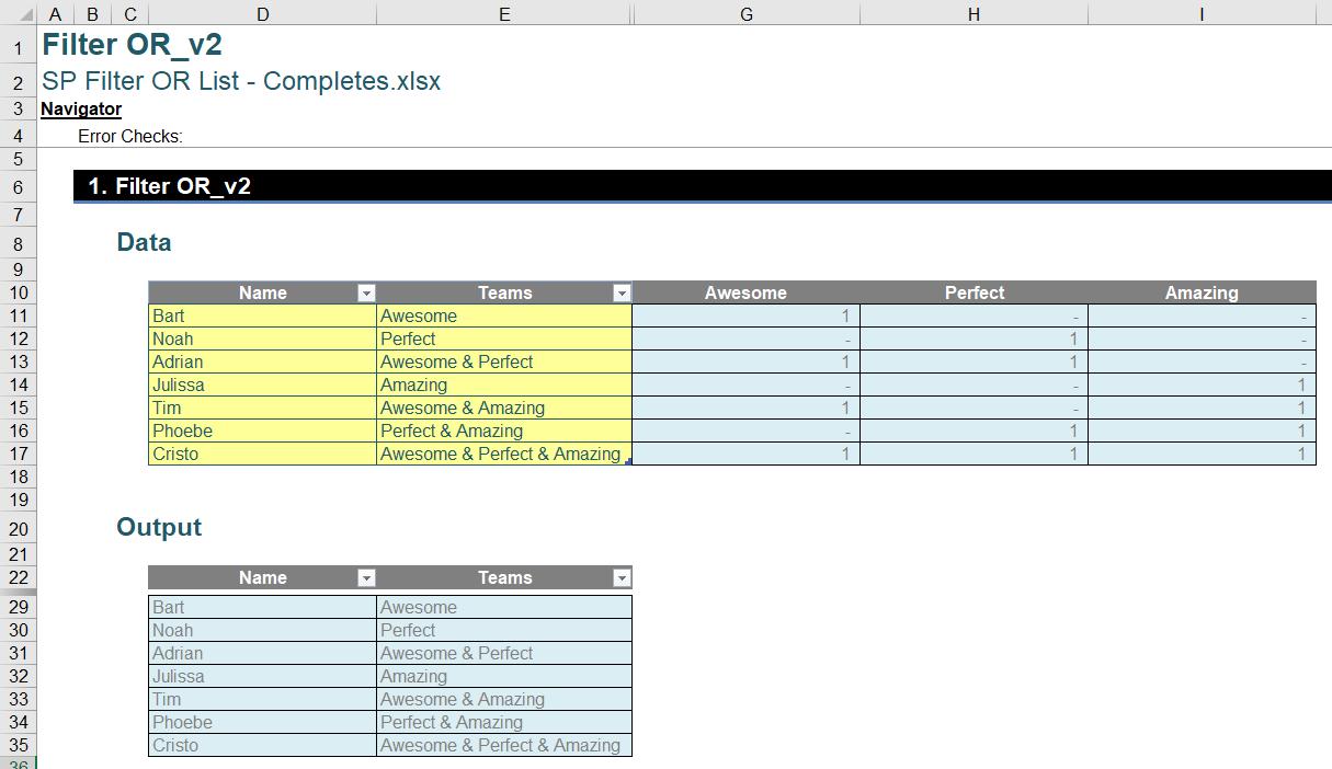
This will use the Included column in the Data_v1 table to filter out all of the matches we have on the Data_v1 table and output it out in the form of an array. Therefore, we have the following output table:
It is important to note that anything typed below a Table will automatically add a new row to the Table. Therefore, you may need to resize the Output table to exclude the new formula that was just added.
Hide, but not completely
The project is currently 80% complete, but we need to hide rows 23 to 25 from our output. However, we need to be careful when hiding these rows. We do not want to completely hide them, as this could cause the SUBTOTAL to become zero [0] or the filter to stop working.
The lowest pixel height for a row that will still allow the SUBTOTAL function to work is 1/3 pixel (0.25 points). To achieve this, we can select the rows we want to hide and go to Home -> Cells -> Format -> Row Height (or use the shortcut key Alt + H + O + H) and enter 0.25 points in the box. However, the filter of Excel will not work if cell is under one [1] pixel (0.75 points). Therefore, we need to adjust the row height to one [1] pixel to ensure that our filter works properly.
After setting the row height to one [1] pixel, our filter is now complete:
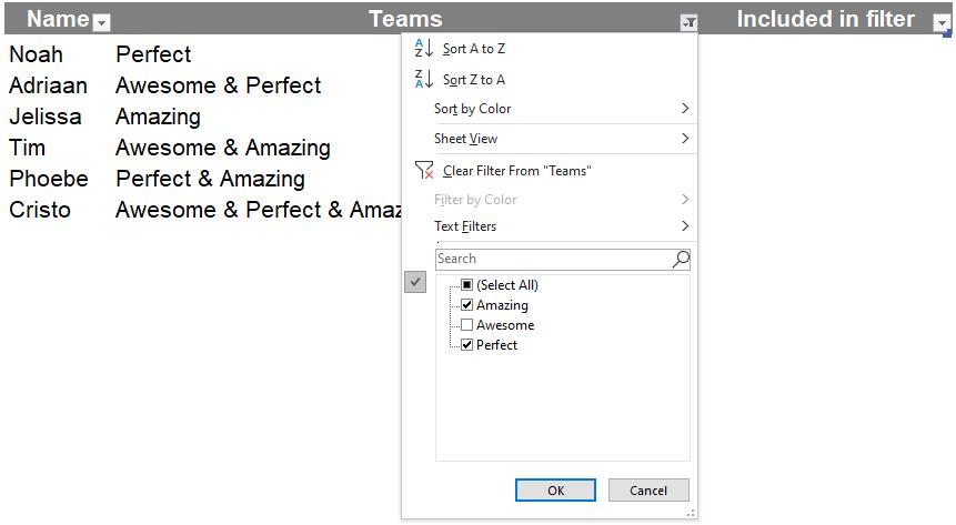
Now, we may use the drop-down menu from the Table to filter out Data_v1[Teams] that contains the keywords we need. The drop-down filter will automatically set the row height to zero [0] pixels for unselected criteria and maintain one [1] pixel for selected criteria.
Suggested Solution 2
The first solution is effective, but is constrained in terms of scaling ability. Therefore, we have another solution to offer to users that can use the LAMBDA function and dynamic arrays. To do this, we will alter few formulae and steps here to make our solution more dynamic and able to absorb more inputs such as a list of keywords that we want to be able to filter by.
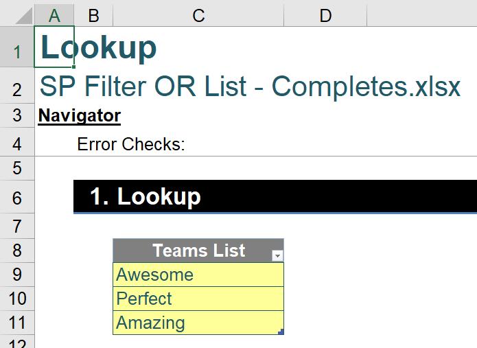
First of all, we create a Look Up table on the Lookup sheet for Teams, we will name this table LU_Teams:
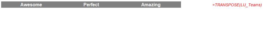
Next, we create our dynamic heading from these inputs by using the following formula:
=TRANSPOSE(LU_Teams)
As our inputs are in rows but we want our headings across the conditionally formatted columns we will need to transpose our inputs:
Next, we need to construct a matrix that will tell us which of the keywords Teams contains using this formula:
=ISNUMBER(SEARCH($G10#,Data_v2[Teams]))*1
This formula uses the dynamic headings (in the range G10#) as the find_text argument and the Teams column in the Data_v2 table as the within_text argument of the SEARCH function. Since G10# is a column vector and the Teams column is a row vector, the formula will search for the first keyword, which is ‘Awesome’, in every item in the Teams column and output it to the first column of the matrix then it proceeds to the second keyword and outputs this to the second column of the matrix and the same for the third keyword and third column of the matrix. After the search, we will have a matrix of integer numbers, wrapping this within the ISNUMBER function will convert these to logical values and then multiplying by one [1] will create a matrix of one [1] and 0 [zero] values, as with solution 1.
Next to the output, instead of using the Table here we will use Dynamic Arrays to create the filter. In cells D22:F22 we create the same headings as we did in solution 1:
In cell E23 we enter the following formula:
=LU_Teams
This creates the keywords lookup in form of a row vector.
In cell F23 we will need a formula that is able to spill down if we have more keywords added in the LU_Teams table. However, it will be hard without using a recursive function like LAMBDA here as SUBTOTAL doesn’t create arrays. Thus, we will use the following formula to create a Dynamic Array that uses SUBTOTAL:
=BYROW(E23#,LAMBDA(row,SUBTOTAL(103,row)))
As we know from solution 1, this part of the formula is the main engine of our filter:
SUBTOTAL(103,row)
This portion of the formula will use an input (called row here) and apply that input as the second argument of our SUBTOTAL function. The final function, which is BYROW, will help us dissect the matrix into multiple rows and feed these into the row parameter of the LAMBDA function. The LAMBDA function will treat each of those row array inputs individually and apply the SUBTOTAL function to each, outputting an array of SUBTOTAL. After typing the formula in cell F23 we will have a dynamic array of SUBTOTAL results that behave similarly to our formulae in solution 1.
The next step here would be using the FILTER function, similarly to our approach in solution 1, in cell D29 we enter the following formula:
=FILTER(Data_v2,MMULT(G11#,F23#),"")
The MMULT function here will multiply the matrix we created within the range G11# by the row vector we created in the range F23#. This would result in a row vector outlining which rows contain the applicable keywords under the current filter context. Our Table is then filtered based on this result.
The last step here is to apply the filter, we simply select D22:F27 then click Home -> Editing -> Sort & Filter -> Filter (or Alt + H + F + S for short). Then we hide column F and set row 23 to row 28 to one [1] pixel. Voila, we have a scalable filter for this challenge!
Word to the Wise
We appreciate there are many, many ways this could have been achieved. If you have come up with an alternative, radically different approach, congratulations – that’s half the fun of Excel!
The Final Friday Fix will return on Friday 25 August 2023 with a new Excel Challenge. In the meantime, please look out for the Daily Excel Tip on our home page and watch out for a new blog every business working day.