Monday Morning Mulling: May 2025 Challenge

On the final Friday of each month, we set an Excel / Power Pivot / Power Query / Power BI problem for you to puzzle over for the weekend.  On the Monday, we publish a solution.  If you think there is an alternative answer, feel free to email us.  We’ll feel free to ignore you.

The Challenge

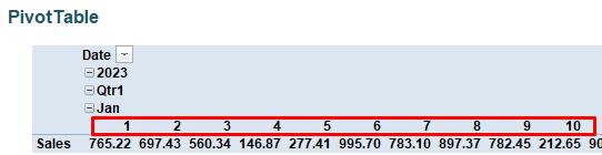
Last Friday’s challenge invited you to create a PivotTable that provides the date of the month only when displaying dates, viz.

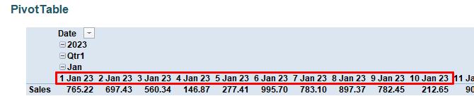
to this:

A Table (called Inputs) was provided containing a set of dates and sales you may use to create your PivotTable:

You can download the original question file here. 

These were the challenge guidelines, you could:

• use PivotTables only
• not use conditional formatting
• not use Excel formulae
• not use VBA, Office Scripts or any other programming code.

Suggested Solution

You can find our Excel file here.  which shows our suggested solution.  The steps are detailed below.

This Final Friday Fix sounded simple.  However, as you might have already realised, finding the right feature within Excel to complete even simple tasks can sometimes be tricky.

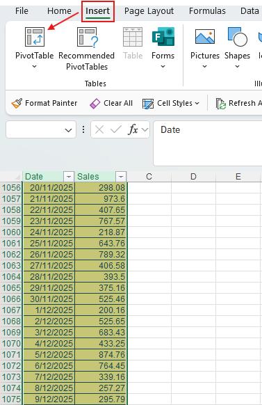
First, we need to construct the PivotTable.  Select any cell in the ‘Data’ table, then go to the Insert tab and click the PivotTable icon:

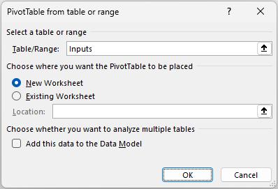
…and press OK:

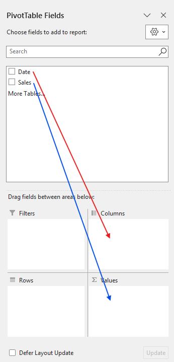
You will see the PivotTable Fields pane on the right-hand side.  Drag the ‘Date’ field (red) into Columns and the ‘Sales’ field (blue) into Values:

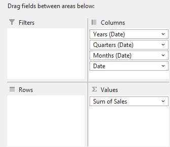
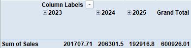
This will be the result, showing both the PivotTable Fields and the constructed PivotTable:

(Some versions of Excel will automatically replicate the numerical formatting of the source data.  The version used above did not, but it is easy to change the Vales number formatting – that is not the challenge!!)

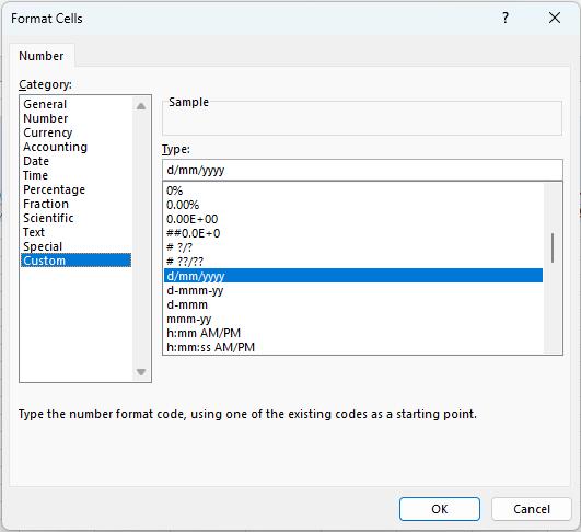
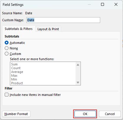
Now, on the PivotTable Fields pane, click on the ‘Date’ heading under Columns. Click on ‘Field Settings…’ and then ‘Number Format’ in the ‘Field Settings’ dialog box:

Then click on Custom:

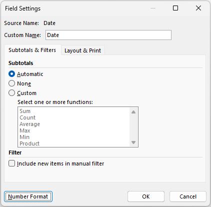
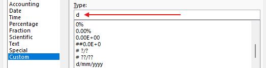
…and change the current date formatting (d/mm/yyyy) under Type to just ‘d’:

Then click OK and OK again.

which will produce the desired date format, only displaying the day:

The trick here is to format the ‘Date’ field.  If you select a different field, the formatting will not “stick” – hence the challenge.

This concludes this month’s challenge.  Sometimes, Excel can feel like a maze to navigate even for simple tasks, luckily, we’re here to help!

The Final Friday Fix will return on Friday 27 June 2025 with a new Excel Challenge.  In the meantime, please look out for the Daily Excel Tip on our home page and watch out for a new blog every business working day.