Monday Morning Mulling: September 2022 Challenge

On the final Friday of each month, we set an Excel / Power Pivot / Power Query / Power BI problem for you to puzzle over for the weekend.  On the Monday, we publish a solution.  If you think there is an alternative answer, feel free to email us.  We’ll feel free to ignore you.

The challenge this month was to extract a name from a text string that contains special characters. 

The Challenge

There may be a time when you are using Excel that you wish to extract a name of a person from a churn of endless text strings that has all sorts of characters that you have never seen or used before.  We gave you a similar challenge here, you can download the question file here.

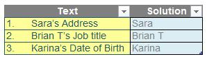
This month’s challenge was to write a formula to extract the name of a person from a text string.  The result should look like as picture (below):

As always, there were some requirements:

• the formula needed to be within just one column (no “helper” cells)
• this was a formula challenge; no Power Query / Get & Transform or VBA!
• the formula should be dynamic enough when a similar text string was added.

Suggested Solution

You can find our Excel file here which demonstrates our suggested solution.

Before we discuss the solution, I would like to note there are several complicating factors here.  Let’s go through them.

Problem 1: The Unremovable White Space

When tackling this problem, we might rely on some functions like TRIM and CLEAN to clear the text.  The TRIM function helps us strip extra white space from the text leaving only a single space between words and no space characters at the start or end of the text.  The CLEAN function helps us remove all nonprintable characters from text.  Thus, using the TRIM and CLEAN functions might help us remove all unwanted white spaces and nonprintable characters:

In the formula above, Text is the name of the table.  Therefore, Text[@Text] specifies one row of column Text, where the above formula is located.  However, these two functions do not appear to work with these text strings no matter how many times these functions apply: the white space is still there.  This is because there are some special invisible characters that the TRIM and CLEAN function cannot remove.  Hence, using TRIM and CLEAN functions for this challenge will not solve our problem.

Problem 2: The Unfindable Apostrophe

The FIND function is quite useful here to address the challenge.  It may help us look for the position of a character within the text string.  Moreover, the target text we need to extract is between the white space and the apostrophe, so FIND can give us the location of those items which can, later on, be used to extract the target text.

However, you might run into the problem that the FIND function results in the #VALUE! error when you try to search for the apostrophe.  This is because there is a “weird” apostrophe within the text string which is different from the normal apostrophe on the keyboard.  Therefore, the FIND function must be tweaked to be able to search for that apostrophe in the text string.

Brainstorming

To address the unremovable white space and unfindable apostrophe problems, we will need a quick inspection of the text string to fully understand it.  Therefore, we will transform each letter of the text string into individual cells in the spreadsheet.

For Microsoft Excel 365 and online versions, we may use Dynamic Arrays with the following formula:

SEQUENCE(1, LEN(Text[@Text])) will help us create a horizontal list of the consecutive text string from one [1] to the last number which is equal to the length of the string.  For example:  

The MID function will then extract each character of a string with the starting point one by one, equal to the number list created by SEQUENCE above.

After you copy down the formula, the result should look like this:

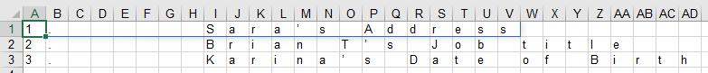
We can see that there are many invisible characters and white space at the beginning of the strings.

Next, we will need to identify what those invisible characters are.  We can use UNICODE and UNICHAR functions to our Dynamic Arrays above.  UNICODE allows us to return numeric code for the first character in a text string.  UNICHAR translates that code back into a character.  (You can also use CODE and CHAR functions here,  but we suggest using UNICODE and UNICHAR as some special characters are not in the database of CODE and CHAR).  The formula to return numeric code is as follows:

  The result is as follows:  

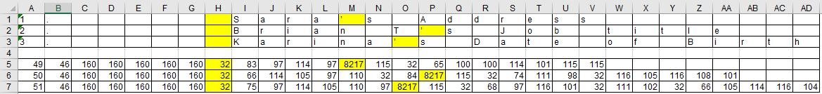
Upon inspection, we can see that the codes of these “invisible characters” are 160 and 32.  Unicode 32 is our normal “Space” generated by pressing the spacebar on the keyboard, while 160 is the “No-Break Space”, generated by pressing ALT + 0160.

For the normal “Apostrophe” that we use on the keyboard, they have the Unicode of 39, while the apostrophe used in the text string is the “Right Single Quotation Mark” which has the Unicode 8217.

Back to the Suggested Solution

As we can see here, all 3-text strings have 32 in front of the target name and 8217 at the end of the target name.  So, we can write a FIND function to find their position of them. 

This situation is perfect to extract the key data from the text string as FIND function will give out the position of the first appearance of the letter.  So, if we use FIND function on the “No-Break Space” character that has Unicode 160, it will result in three [3] which is not a desirable starting position.

Hence, the starting position of the target text should be:

and the number of characters we extract is:

From here we can use the MID function to extract the target text as follows:

See you next month!

The Final Friday Fix will return on Friday 28 October 2022 with a new Excel Challenge.  In the meantime, please look out for the Daily Excel Tip on our home page and watch out for a new blog every business working day.