
Monday Morning Mulling: September 2023 Challenge
2 October 2023
On the final Friday of each month, we set an Excel / Power Pivot / Power Query / Power BI problem for you to puzzle over for the weekend. On the Monday, we publish a solution. If you think there is an alternative answer, feel free to email us. We’ll feel free to ignore you.
The Challenge
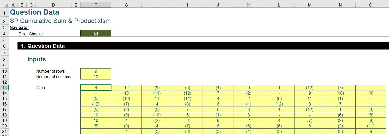
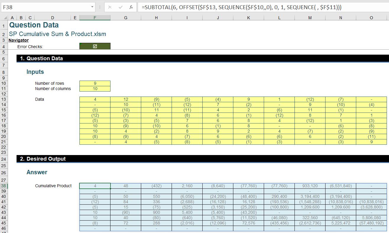
Last Friday, we challenged you to produce row cumulative sums for a 9×10 numeric array using only one [1] Excel formula, and to produce row cumulative products for the same array with, again, “just” one [1] formula. You could download the question file here.
The outputs were to look like the following upon completion:
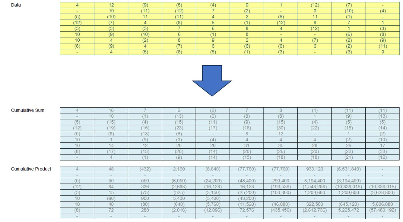
There were some requirements:
- each formula needed to be within one cell
- the function LAMBDA and any of its helper functions (e.g. LET, BYROW or MAP) were not allowed
- this was a formula challenge; no Power Query / Get & Transform or VBA.
Suggested Solution
You can find our Excel file here, which shows our suggested solution. The steps are detailed below.
The OFFSET Approach
The OFFSET function has four [4] arguments:
=OFFSET(reference, rows, columns, [height], [width])
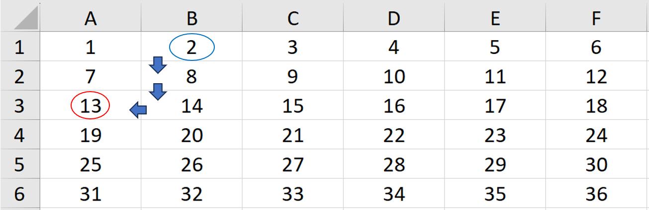
The argument reference accepts a cell or range of adjacent cells, and it is the base of the OFFSET. The arguments rows and columns are displacements from reference, i.e. the number of rows downwards and the number of columns to the right. They accept both positive and negative values, and negative values simply represent movements in the opposite direction. For example,
=OFFSET(B1, 2, -1)
would take us two [2] rows down and one [1] column to the left, ending up at cell A3.
The optional arguments height and width are dimensions of the output array from reference after displacement, and they only accept positive values. Again, height and width are measuring downwards and to the right, and they both have a default value one [1]. We have an article with more details on the OFFSET function here.
Increasing the width argument of an OFFSET formula applied on the input array whilst keeping height as one [1] will produce longer and longer one-row segments from the input. This way, we can extract “running segments” from the array.
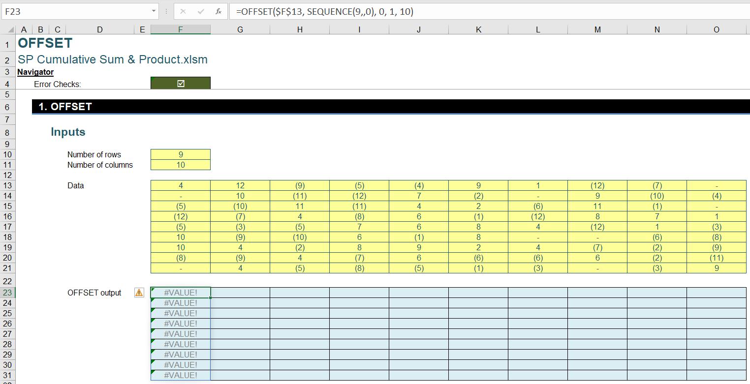
For example, from the top-left corner (F13) of our input array, if we specify a width of one [1]
=OFFSET(F13, 0, 0, 1, 1)
then we are outputting the cell F13 itself. If we then specify a width of two [2]
=OFFSET(F13, 0, 0, 1, 2)
then we are outputting a spilled range F13:G13, the first two [2] cells in the first row of our input array. Following this idea, we can increase the width argument in the OFFSET to sequentially spill “running segments” of a row. For example, a width of nine [9] will give us the first nine cells in the first row (F13:N13):

Hopefully, it is intuitive at this point that, if we can find a way to output all “running segments” with one [1] formula and output the totals of these spilled ranges instead of spilling them, we will obtain an output row of running totals.
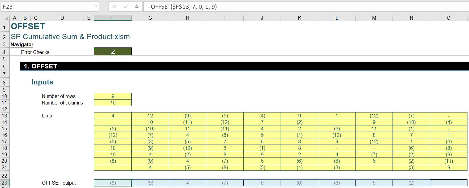
The Rows Argument
Before implementing the above idea, let’s look at the rows argument in the OFFSET function and how we may cover all rows of the input array. The rows argument is the vertical displacement from reference, i.e. the number of rows downwards. Using the top-left corner F13 as the reference and increasing rows from zero [0] to eight [8], we can output from the first row to the ninth, or the last row of the array. For example, with a rows value of seven [7] and a width value of nine [9], we can output the first nine [9] cells of the second last row (F20:N20):
What we need to do next is to figure out how to output all “running segments” of each row and all rows with only one [1] OFFSET formula. We also need to find a way to sum for each of the output spilled ranges.
However, OFFSET doesn’t work well with array inputs if we try to be dynamic with either width or rows. For example:
The Excel engine allows some functions to spill, but not others due to limitations with the prohibition of creating arrays of arrays.
Even if we obtained an array of spilled “running segments” as planned, we couldn’t simply use SUM or PRODUCT to produce running totals or running products from those “running segments”. The reason is that SUM and PRODUCT are aggregate functions, and they will produce one [1] output aggregating (adding / multiplying) everything in one [1] cell, instead of preserving the array structure.
So far, the intermediate output before addition or multiplication we can visualise to have the structure of an array with spilled rows or spilled “running segments”. In the OFFSET we will be using numbers one [1] to 10 for width, and zero [0] to eight [8] for rows.
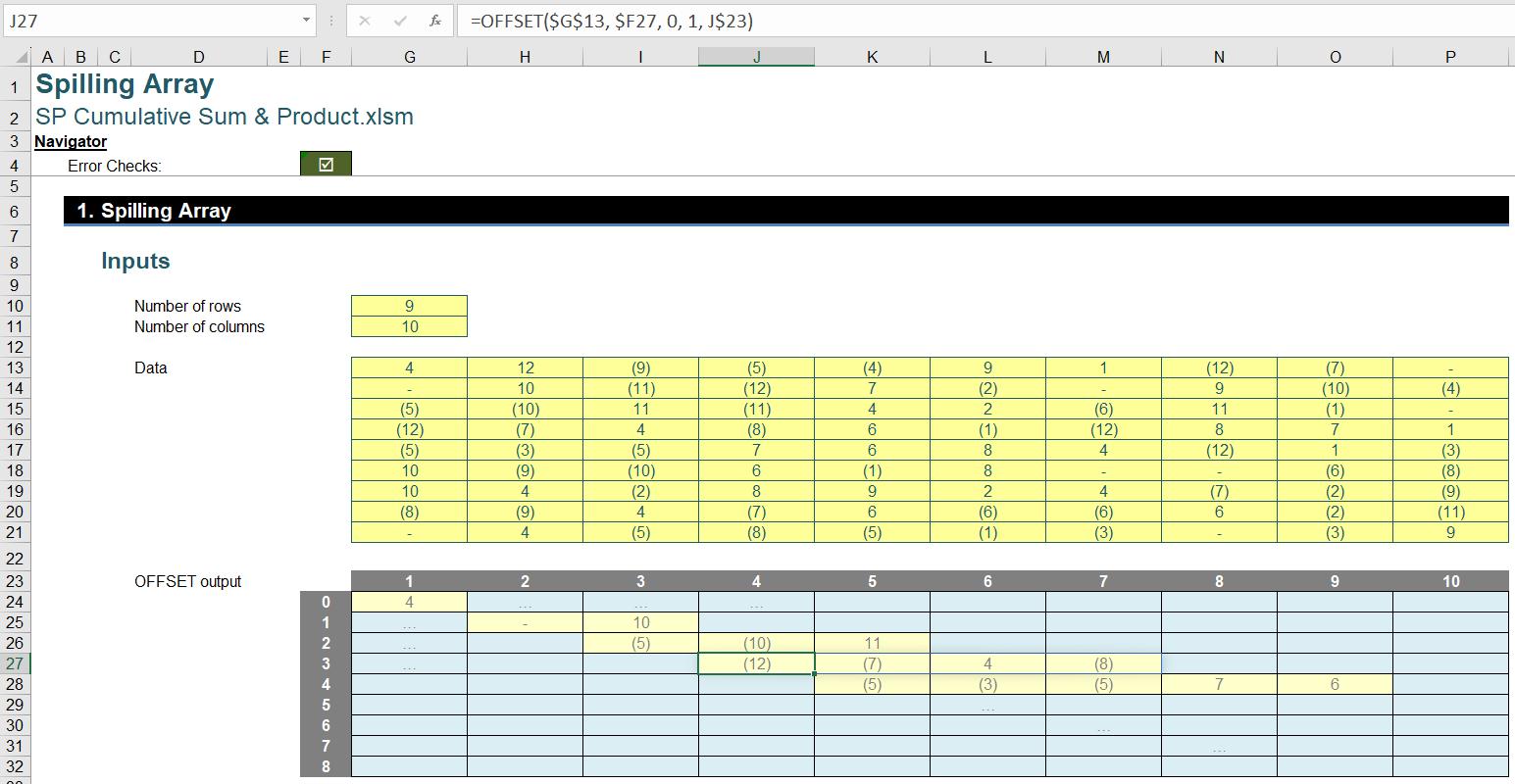
In the above illustration, we haven’t filled up the array but only showed a few spilled segments, so we don’t bother you with a fullscreen of #SPILL! errors.
A SUBTOTAL Structure
Now here is where the function SUBTOTAL comes into play. It has the following syntax:
=SUBTOTAL(function_number, reference1, [reference2], …)
The first argument function_number specifies the function to perform. For example, one [1] is AVERAGE and nine [9] is SUM.
If we use outputs from OFFSET as the reference inside a SUBTOTAL, we are allowed to use arrays as width and rows for the OFFSET. Moreover, SUBTOTAL performs quite similarly to BYROW or MAP, that it executes the specified function on each reference, and preserves the array structure instead of aggregating everything like SUM or PRODUCT.
We can design a two-dimensional structure using SEQUENCE to cover the whole array. We first use a horizontal sequence of length ten [10] in width to produce “running segments” of a row:
=SEQUENCE(, 10)

Then we use a vertical sequence of length nine [9] but starting from zero [0] in rows, to cover all nine [9] rows of the array:
=SEQUENCE(9, , 0)
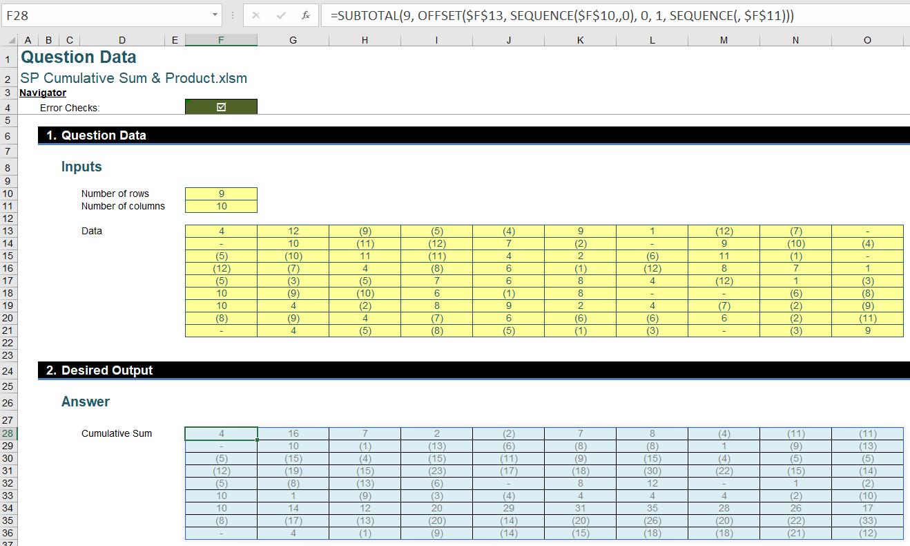
For running totals, we can combine the above inside OFFSET and SUBTOTAL, and specify a function_number nine [9] for SUBTOTAL:
=SUBTOTAL(9, OFFSET($F$13, SEQUENCE($F$10, , 0), 0, 1, SEQUENCE(, $F$11)))
and the output will be a dynamic array of row running totals for the input array:
Similarly, specifying a function_number of six [6] for SUBTOTAL produces a dynamic array of row running products for the input array:
=SUBTOTAL(6, OFFSET($F$13, SEQUENCE($F$10, , 0), 0, 1, SEQUENCE(, $F$11)))
Thus, we achieve to produce arrays of row running totals and row running products with only one [1] Excel formula for each. We also encourage you to play around with other functions in SUBTOTAL. For example, running maximum and running minimum will be both interesting and useful.
The Final Friday Fix will return on Friday 27 October 2023 with a new Excel Challenge. In the meantime, please look out for the Daily Excel Tip on our home page and watch out for a new blog every business working day.