Monday Morning Mulling: September 2024 Challenge

On the final Friday of each month, set an Excel for you to puzzle over for the weekend.  On the Monday, we publish one suggested solution.  No-one is stating this is the best approach, it’s just the one we selected.  If you don’t like it, lump it – or contact us with your preferred solution.

The Challenge

On Friday, we gave you another bold challenge that sounds simple but requires some thought.

We asked you to consider the following:

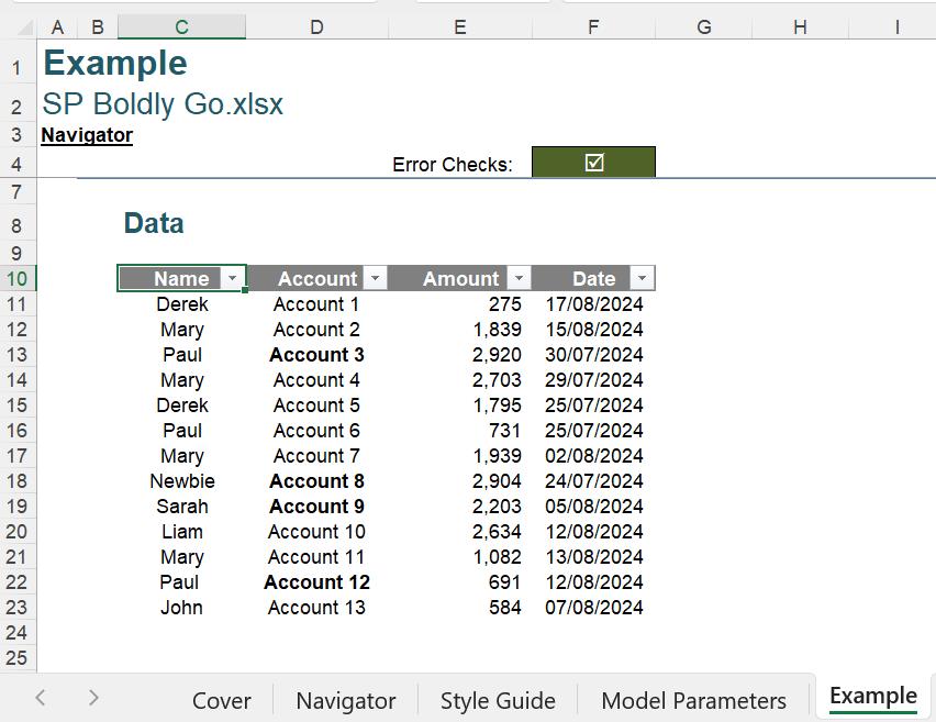
You can download the original question file here.  We have a list of accounting data, where some of the Account data is shown in bold case.  We need to filter the data so that only the rows with bold account codes are shown.

This month’s challenge was simple.  You had to solve it as simply as possible, with no Preview features, VBA or Power Query.  This is a deceptively simple Excel challenge!

Suggested Solution

The colourful key to solving this month’s challenge is not to apply some advanced filtering, but to consider how we can manipulate the bold text so we may use the simple filter functions to achieve our goal.

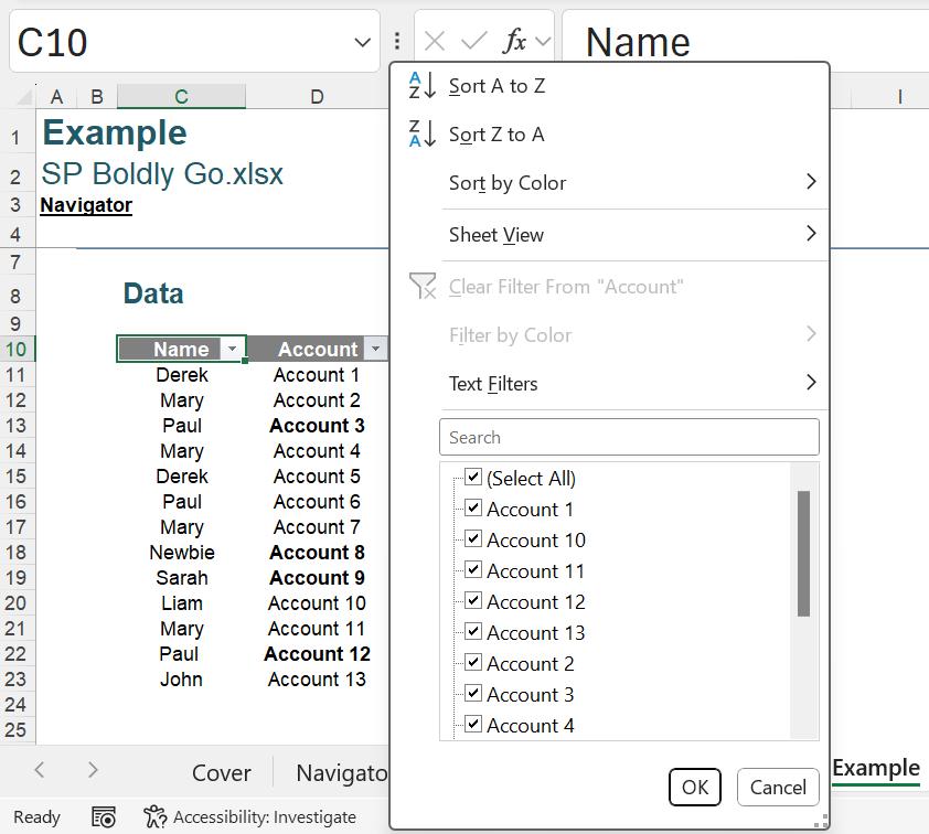
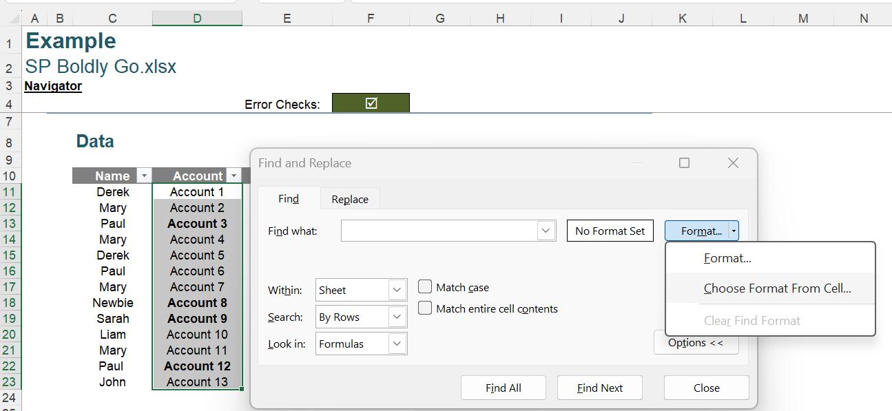
It may not be possible to ‘Filter by Bold’, but there is an option to ‘Filter by Color’.  We can do this by using the Find functionality.  Let’s begin by selecting the data in the Account column and using the shortcut CTRL + F to show the ‘Find and Replace’ dialog. 

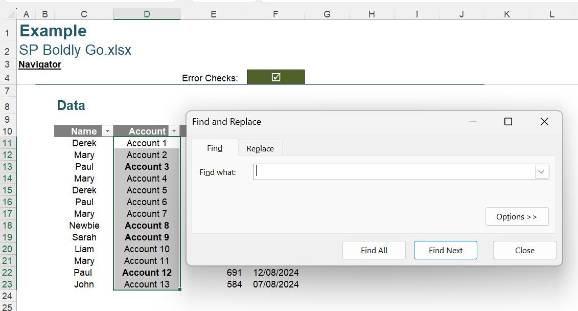
Since we want to find a cell format and not a value, we need to use the Options button to see what other functionality is available:

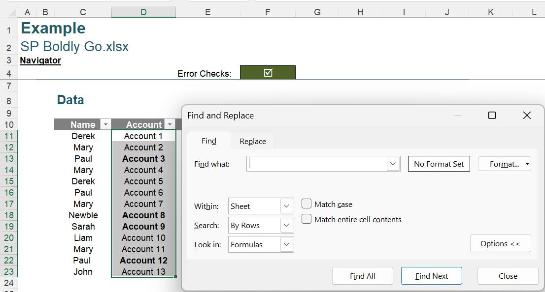
Using the Format button, we may determine the format to be found from a cell:

If we select one of the cells with bold text, a Preview of the formatting is shown:

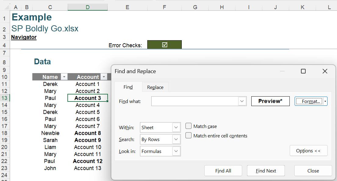
We may now ‘Find All’:

The next step is to replace the formatting with a colour.  There are two [2] ways to do this. 

Replace formatting with Replace tab

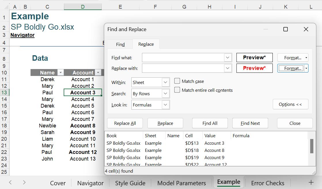
On the Replace tab, we may replace the formatting.   This time we show the ‘Format…’ option.  This is the option we would have chosen in the Find tab if it had been difficult to locate a bold cell to copy. 

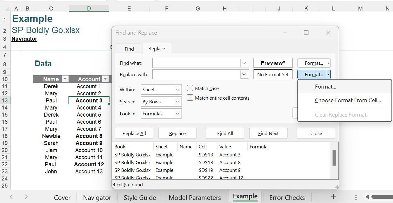
In the ‘Replace Format’ dialog, we may choose from any cell format:

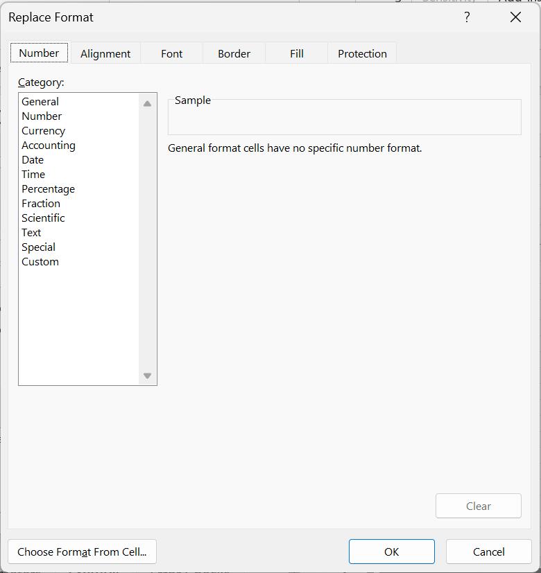
For our example, we would like to change the font, therefore we access the Font tab and choose a colour.  We also make the new font bold too:

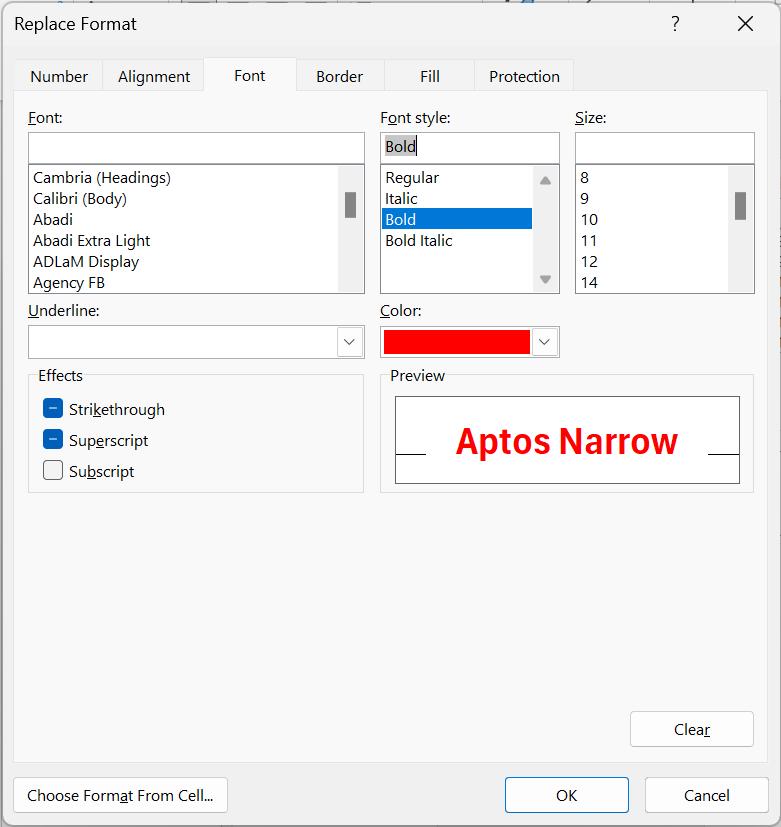
We click OK, we are shown the Preview for the replacement:

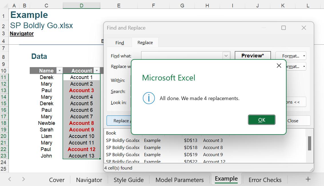
We ‘Replace All’ and the bold font is now red:

Replace font using CTRL + A

There is a simpler method we could use for this example.  Starting from the point where we found the rows that had bold text:

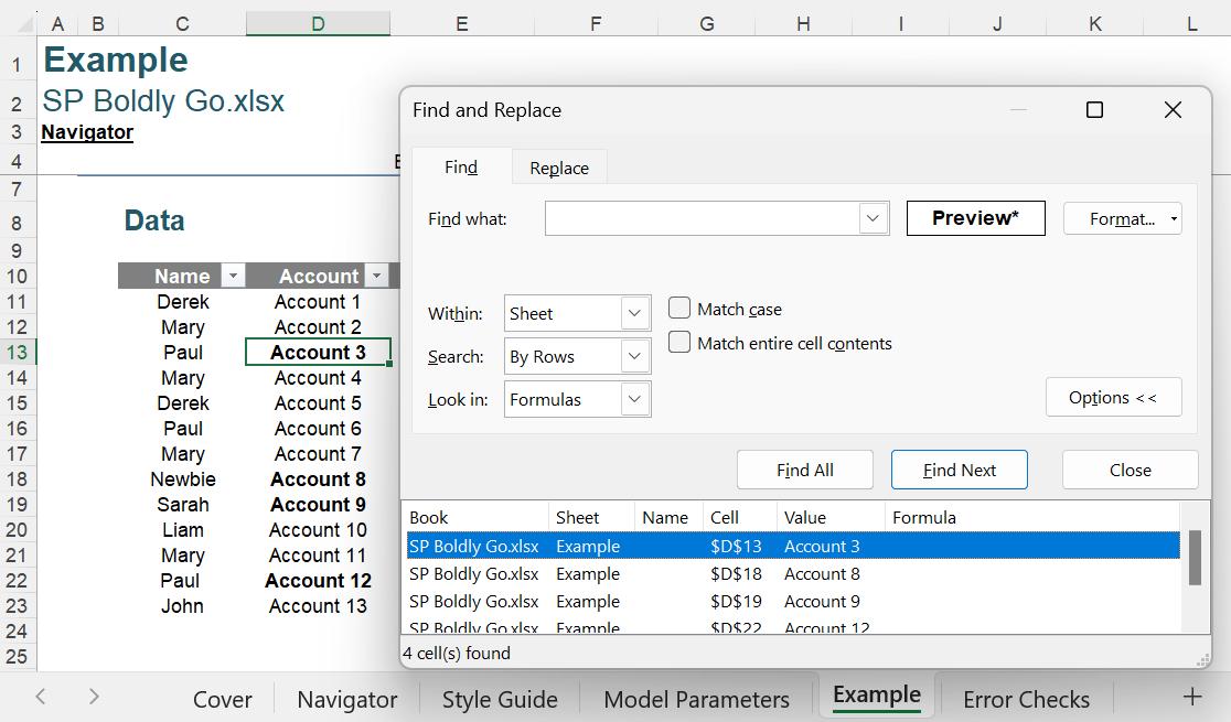
If we use CTRL+ A, we select all the cells with bold formatting:

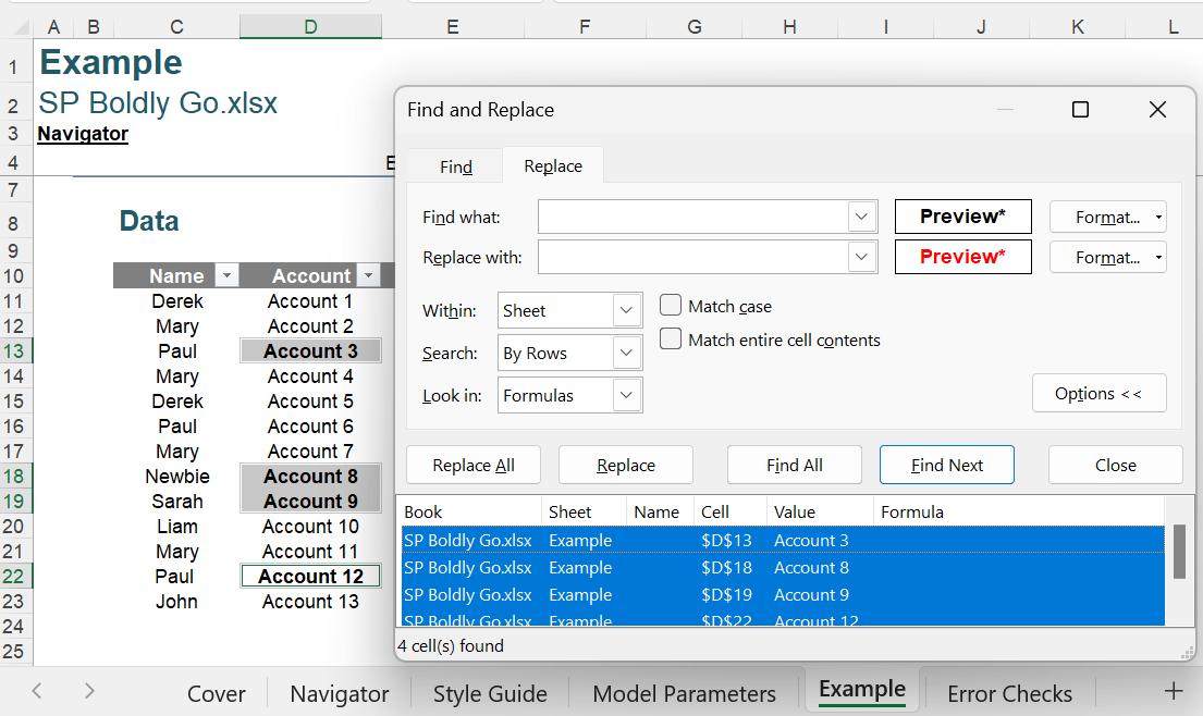
We may then change the colour on the selected cells from the Home tab:

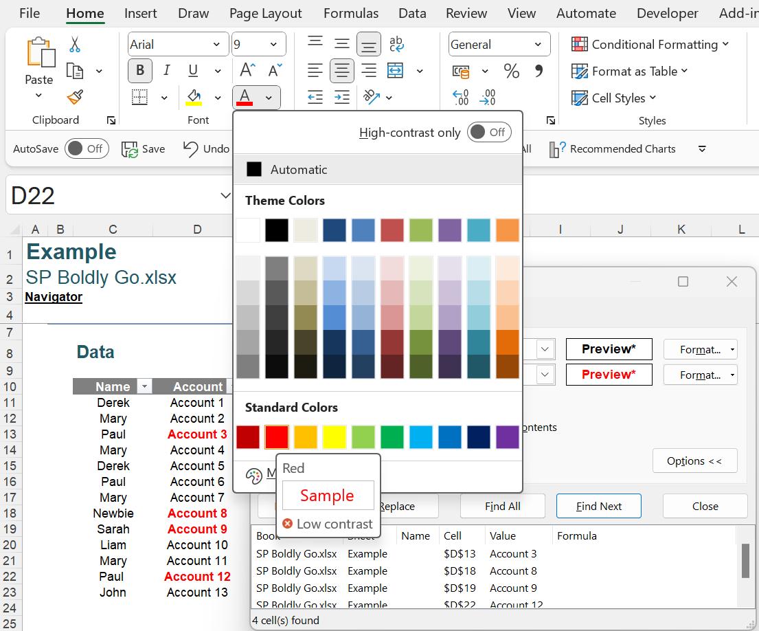
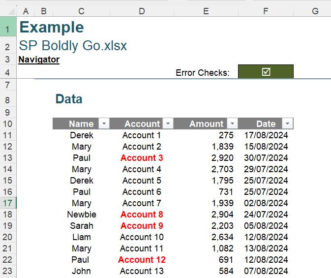
Using either method, we now have the bold text in red:

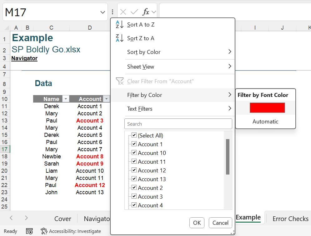
Now, we may use the filter button on the Account heading to filter on the bold text:

The data has been filtered as required:

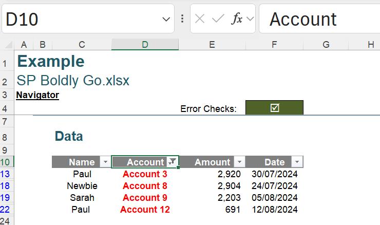
Problem solved.  The solution file may be inspected here.

The Final Friday Fix will return on Friday 25 October 2024 with a new Excel Challenge.  In the meantime, please look out for the Daily Excel Tip on our home page and watch out for a new blog every business working day.