Monday Morning Mulling: December 2016
2 January 2017
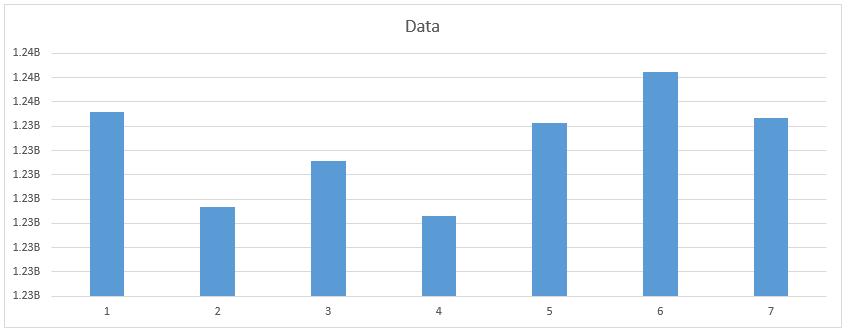
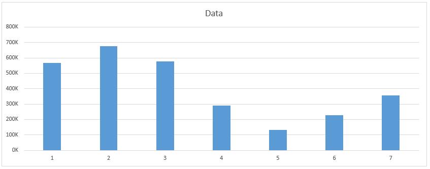
Welcome again to 2017! Last week, at the end of December, we asked if you could create a chart that would have the number format of the chart axis dynamically change when the values being charted increase or decrease.
Chart axes will, by default, take on the number formatting of the cells in the first data series that it uses. This means that if you set the number formatting in the data cells, you can have up to three different number formats built into the cell. However, if you use conditional formatting to get the fourth format, the conditional formatting doesn’t flow onto the chart!

The Solution
The trick here is to take advantage of one of the perennial black sheep in Excel. The OFFSET function, amongst its other neat features, can be used inside a named range to create a dynamic range that can select different rows depending on a condition that we set up. So, if we set up 4 rows, each with their own number format, then we can create a named range that chooses which row to get the chart data from.

When you change the numbers, the named range will automatically pick up the correct row, and the chart axis will update in kind.


This is our attempt to find a workaround to get conditional number formatting into the chart axis. By no means are we claiming this is the only way to do it – if you have a more elegant solution, please let us know!

