Monday Morning Mulling: June Challenge

On the final Friday of each month, set an Excel for you to puzzle over for the weekend. On the Monday, we publish a solution. If you think there is an alternative answer, feel free to email us. We’ll feel free to ignore you.

Final Friday Fix: June Challenge Recap

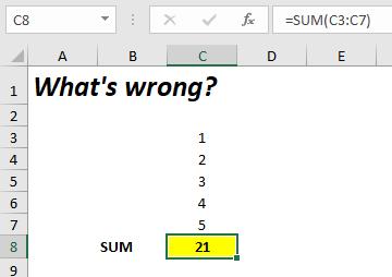
Which came first? The spreadsheet or the SUM function? Who knows and more to the point, who cares? Well, you might care if SUM does not appear to work in a spreadsheet:

The attached Excel file demonstrates this quirk. The question is, how did it happen?

The Solution

Since SUM has been used in models for over 30 years, you are looking in the wrong place if you think the function is to blame. SUM sums numbers, plain and simple. Given there are no hidden rows and columns here, the first thing to check is are the values in cells C3:C7 actually numbers, i.e. do they have a numerical value?

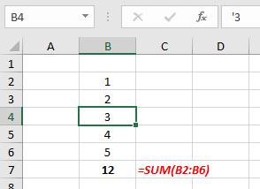
Consider the following example where the number ‘3’ below has been entered as text:

Cell B4 in the above illustration has had an apostrophe added before the value 3.  This makes Excel treat this value as text, not a number.  Text is disregarded in a summation by Excel, therefore the formula

only sums 1, 2, 4 and 5 – the total of which is 12, not 15. 

Extrapolating this idea, this means that the SUM function would produce a total less than the apparent total not more.  Furthermore, the functions VALUE() and N(), both of which consider the value of a cell’s contents suggest nothing is amiss:

Hang on a minute.  Check out that formula in cell K8; it clearly states that cell C8 equals the sum of the above.  Yes, I know that is where we started – but this gives us slightly more information than we had originally in a subtle sort of way.

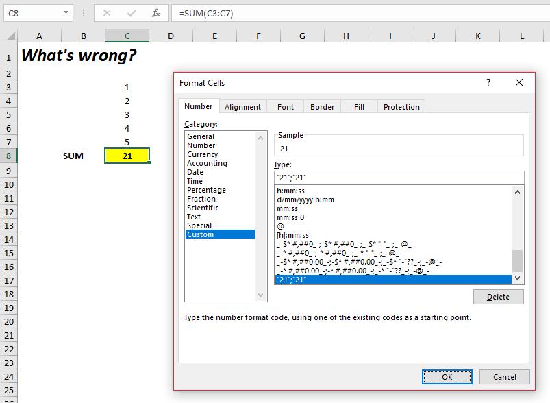
We have determined that cells C3:C8 are all values and that C8 is the sum of the above.  Therefore, it is the appearance of cell C8 that is now in question, not its logic or value.  If you click on cell C8 and then use CTRL + F1 to format cells you discover the following:

Aha!  The cell has been formatted as

Custom number formatting has been used to trick you.  If the number is either non-negative or negative (i.e. it is a number!), the value 21 is displayed regardless of the true numerical value.

Did you spot it?  Well done if you did, but don’t feel too badly if you didn’t.  This example comes from a fraudulent model the author uncovered years ago which conned auditors, investors and a well-known bank out of millions of dollars.  The problem was the model had been audited by auditors but not model auditors – whom possess a different skill entirely. 

You can find out more about custom number formatting here.  If you want to know more about auditing. or believe your model may require a review of some sort, please drop us a line at contact@sumproduct.com.

For more tricks and tips, check out our many examples at www.sumproduct.com/thought.

The Final Friday Fix will return on Friday 28 July with a new Excel Challenge.  In the meantime, please look out for the Daily Excel Tip on our home page and watch out for a new blog every other business workday.