Power BI Blog: Excel-sior Part 2
22 February 2018
Welcome back to Power BI Tips.
Last week we used "Get Data" to import an Excel file, but our data didn't come up nicely in the table. Now it's time to edit the data to get the column headers to come out nicely.
On the Ribbon, under “Home” in the “External data” category, click on “Edit Queries”.

It will bring us into the Query Editor similar to the "Get & Transform"/"Power Query" one in Excel - the colour theme is updated to match Power BI's palette and display our table:

Let’s remove the first row and use the second row as our column headers.
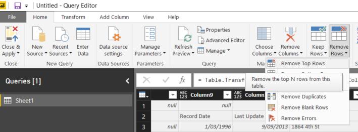
On the Ribbon, under “Home” in the “Reduce Rows” category, click on “Remove Rows” -> “Remove Top Rows”.

A prompt will appear asking for how many, type “1” and hit “OK”

Now on the Ribbon, under “Home” in the “Transform” category, click on “Use First Row as Headers”

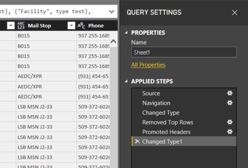
Great! Let’s rename this query to something more meaningful. There are two ways to do this. The first is using the textbox for the Name property in the Query Settings side menu on the right:

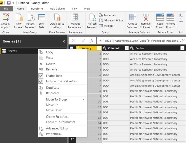
Or right click on the query name in the "Queries" pane on the left and select "Rename":

Tip: you can select the query and press F2 to rename it directly! I’ve renamed it NASA Labs Facilities.
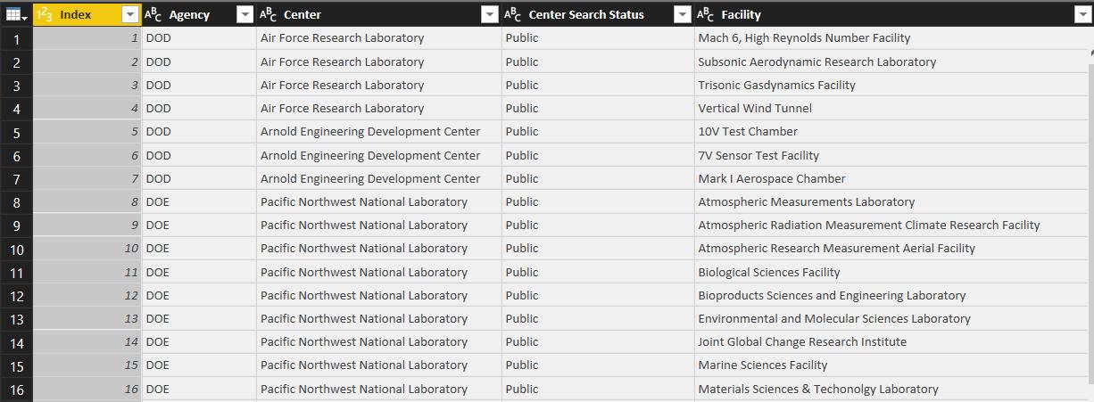
Notice here that the first two columns had a merged cell. The leftmost column is assigned the header but it clearly is an index, with Column2 being the Agency. Rename the columns accordingly.

Hit “Close & Apply” and we are ready to visualise! For the following blog we'll do a basic visualisation with this data.
See you next time for more Power BI Tips.

