Power Pivot Principles: The A to Z of DAX Functions – CHISQ.DIST

In our long-established Power Pivot Principles articles, we continue our series on the A to Z of Data Analysis eXpression (DAX) functions.  This week, we look at CHISQ.DIST function.

The CHISQ.DIST function

In probability theory and statistics, the chi-squared distribution (also chi-square or χ²-distribution) with k degrees of freedom is the distribution of a sum of the squares of k independent standard normal random variables.  It is one of the most widely used probability distributions in inferential statistics, e.g. in hypothesis testing or in construction of confidence intervals. 

The chi-squared distribution is used in the common chi-squared tests for goodness of fit of an observed distribution to a proposed theoretical one, the independence of two criteria of classification of qualitative data, and in confidence interval estimation for a population standard deviation of a normal distribution from a sample standard deviation.

If Z₁, ..., Z_k are independent, standard normal random variables, then the sum of their squares

is distributed according to the chi-squared distribution with k degrees of freedom. This is usually denoted as

Thus, the chi-squared distribution has one parameter: k — a positive integer that specifies the number of degrees of freedom.

As aforementioned, the chi-squared distribution is used primarily in hypothesis testing.  Unlike more widely known distributions such as the normal distribution and the exponential distribution, the chi-squared distribution is rarely used to model natural phenomena.  It arises in the following hypothesis tests, among others.

The primary reason that the chi-squared distribution is used extensively in hypothesis testing is its relationship to the normal distribution.  Many hypothesis tests use a test statistic, such as the t statistic in a t-test.  For these hypothesis tests, as the sample size, n, increases, the sampling distribution of the test statistic approaches the normal distribution (Central Limit Theorem).  Since the test statistic (such as t) is asymptotically normally distributed, provided the sample size is sufficiently large, the distribution used for hypothesis testing may be approximated by a normal distribution.  Testing hypotheses using a normal distribution is well understood and relatively easy.  The simplest chi-squared distribution is the square of a standard normal distribution.  Therefore, wherever a normal distribution could be used for a hypothesis test, a chi-squared distribution could be used.

A chi-squared distribution constructed by squaring a single standard normal distribution is said to have 1 degree of freedom, etc.

The chi-squared distribution is commonly used to study variation in the percentage of something across samples, such as the fraction of the day people spend reading these articles about obscure DAX functions.

The CHISQ.DIST function employs the following syntax to operate:

The CHISQ.DIST function has the following arguments:

• x: this is required and represents the value at which you want to evaluate the distribution
• deg_freedom: this is also required.  This denotes the number of degrees of freedom
• cumulative: this is another mandatory argument.  This is a logical value that determines the form of the function.  If cumulative is TRUE, CHISQ.DIST returns the cumulative distribution function; if cumulative is FALSE, it returns the probability density function.

It should be further noted that:

• if any argument is nonnumeric, CHISQ.DIST returns an error
• if x is negative, CHISQ.DIST returns an error
• if deg_freedom is not an integer, it is rounded
• if deg_freedom < 1 or deg_freedom > 10^10, CHISQ.DIST returns an error
• this function is not supported for use in DirectQuery mode when used in calculated columns or row-level security (RLS) rules.

Examples

Example 1: The chi-squared distribution for 2, returned as the probability density function using three degrees of freedom. The result is 0.207554.

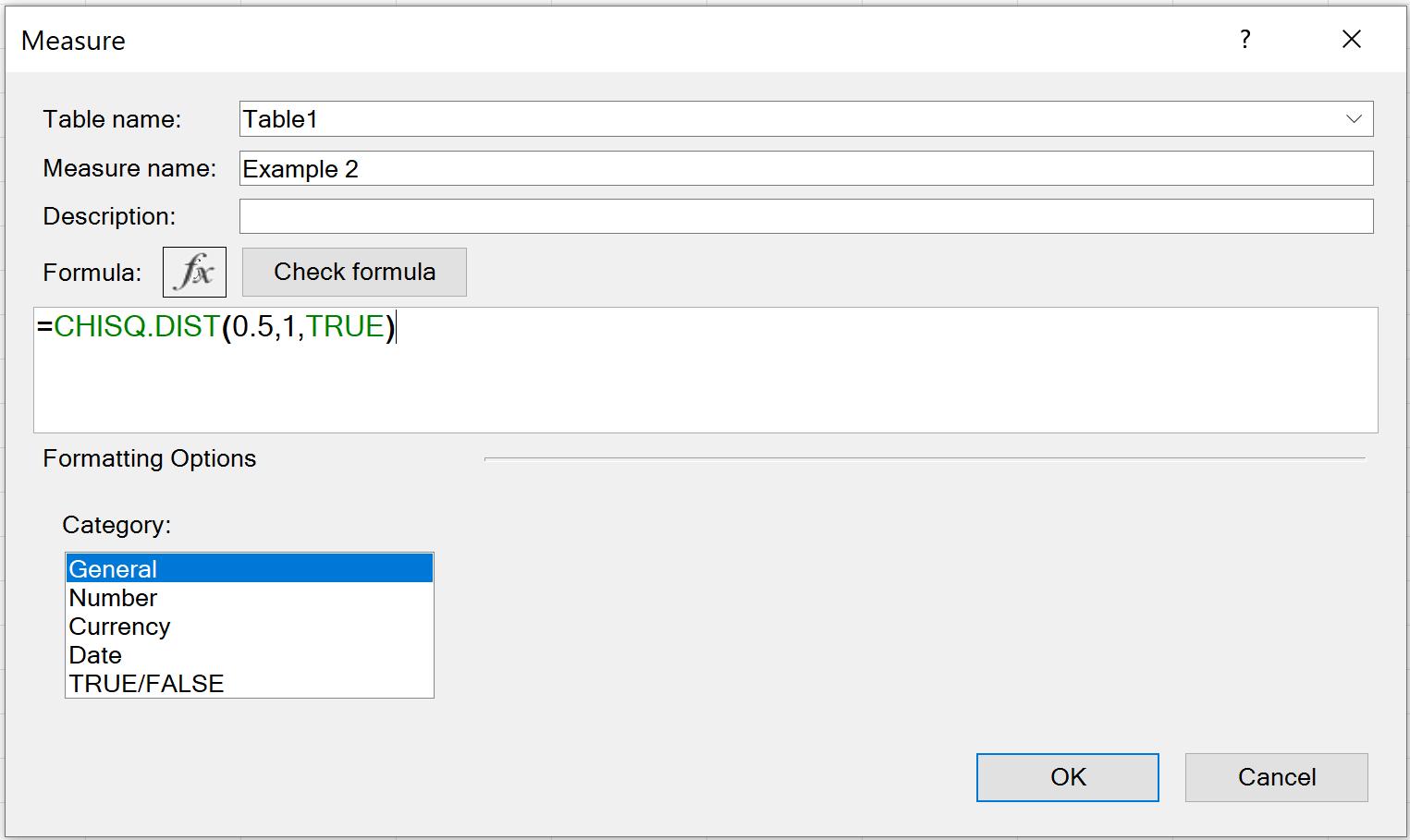
Example 2: The chi-squared distribution for 0.5, returned as the cumulative distribution function using one degree of freedom. The result is 0.5205.

Come back next week for our next post on Power Pivot in the Blog section. In the meantime, please remember we have training in Power Pivot which you can find out more about here. If you wish to catch up on past articles in the meantime, you can find all of our Past Power Pivot blogs here.