Power Pivot Principles: Introducing the DIVIDE Function

Welcome back to our Power Pivot blog. Today, we introduce the DIVIDE function.

A while ago, we ran into the issue of division by zero errors in Power Pivot (you can read about it here). We dealt with that issue with a combination of the IF and BLANK functions to error trap the division by zero errors.

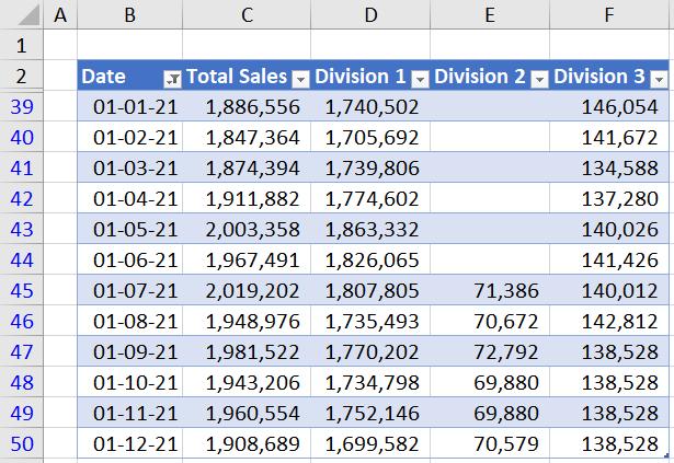
As a quick and dirty example, let’s use the following data:

We get the following PivotTable output:

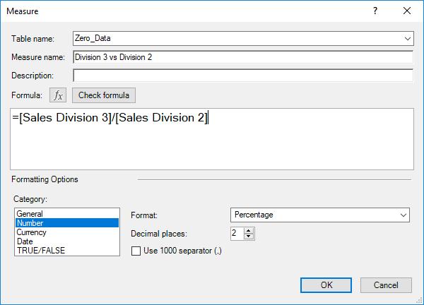
Say we wanted to calculate the percentage difference between the sales in Division 2 and Division 3 using the following measure (assuming that we have aggregation measures for the sales of both divisions):

We get the following PivotTable output:

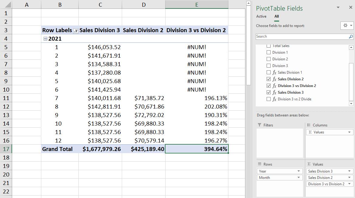
The nasty #NUM! error is caused by the denominator, [Sales Division 2], being zero for those time periods.  Rather than use the BLANK and IF functions to trap these errors, we may use the DIVIDE function instead.

The DIVIDE function uses the following syntax to operate:

The [<alternateresult>] is what the DIVIDE function will return when the denominator is zero (0).  If no value is specified, the default setting is to return with BLANK.

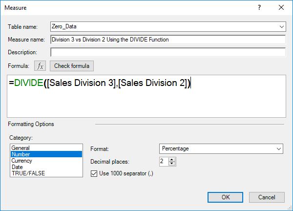
Let’s create a new measure using the DIVIDE function:

This results in the following output from our PivotTable:

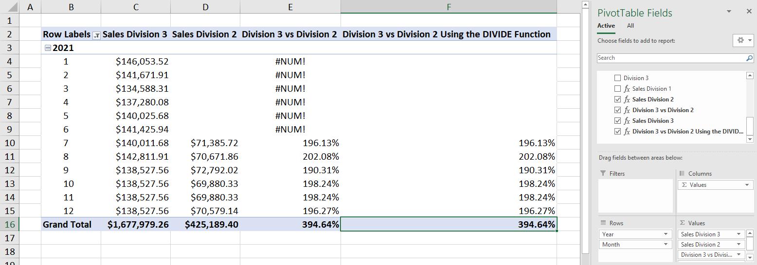
There we go: the DIVIDE function has done our error trapping for us!

That’s it for this week. Until next time, happy pivoting!

Stay tuned for our next post on Power Pivot in the Blog section. In the meantime, please remember we have training in Power Pivot which you can find out more about here. If you wish to catch up on past articles in the meantime, you can find all of our Past Power Pivot blogs here.