Power Pivot Principles: Introducing the PREVIOUSDAY / MONTH / QUARTER / YEAR Functions

Welcome back to the Power Pivot Principles blog.  This week, we will talk about the group of PREVIOUSDAY / MONTH / QUARTER / YEAR functions in DAX.

Previously, we have talked about the SAMEPERIODLASTYEAR function, which returns a table that contains a column of dates shifted one year back in time from the dates referred to in the specified dates column, given the current context.  What if we want a value of one day back, one month or one quarter back?  It’s also good to know about the PREVIOUSDAY, PREVIOUSMONTH, PREVIOUSQUARTER and even the PREVIOUSYEAR functions.

With the same logic, the PREVIOUSDAY function returns a table that contains a column of all dates representing the previous day (funnily enough), in the current context.  The PREVIOUSMONTH and PREVIOUSQUARTER functions also return a table that contains a column of all dates from the previous month or quarter respectively, based upon the first date in the dates column, whilst  PREVIOUSYEAR returns data from the previous year.

These functions follow the syntax:

One thing we should note is that this function determines the first date in the input parameter, and then returns all dates corresponding to the day previous to that first date.  For example, if the first date in the dates argument refers to June 10, 2020; this function returns all dates equal to June 9, 2020.

The dates argument may be a reference to a date / time column, a table expression that returns a single column of a date / time values, or a Boolean expression that defines a single-column table of date / time values.

Let’s consider an example.  Below is [truncated] daily sales data from 2016 to 2019 of a store:

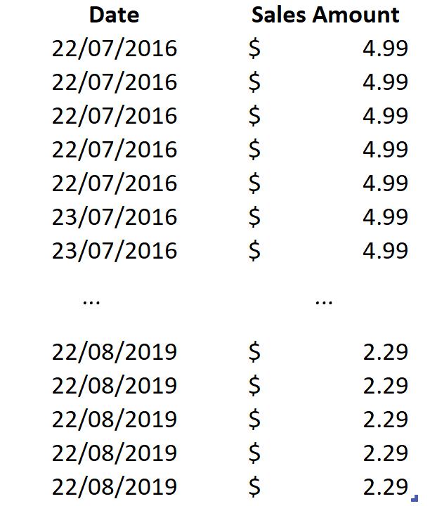
We want to compare sales by each previous date, month, quarter and year.

To do this, we will load the data to the Power Pivot Data Model, by highlighting the whole data, going to the ‘Power Pivot’ tab on the Ribbon and clicking ‘Add to Data Model’. We then rename the tables as Sales. We also add a Calendar Table, which will later be used in our PivotTable, and name it Calendar. We will also define the relationships between Sales and Calendar by switching to ‘Diagram View’ in the Home tab and dragging the Date field to connect the two tables.

Going back to Excel, we create a PivotTable in a new worksheet. Here, we drag Date Hierarchy from the Calendar table into Rows field and Sales into the Values field. Thus, we have a PivotTable showing Sales over time:

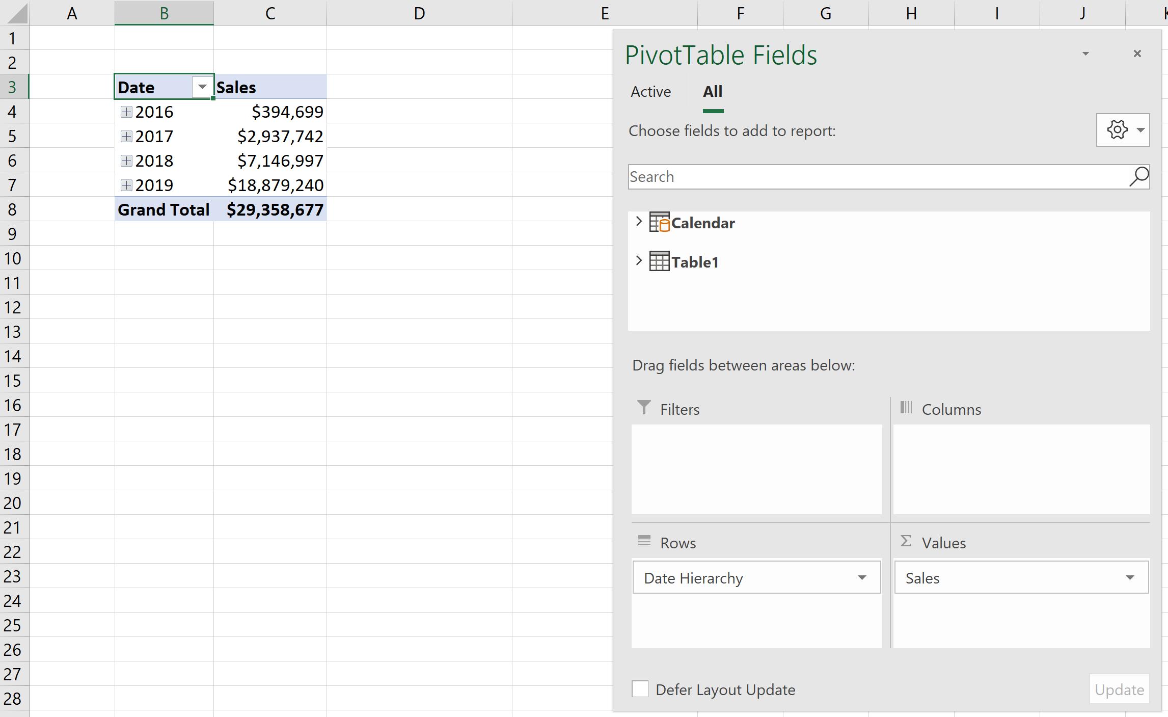
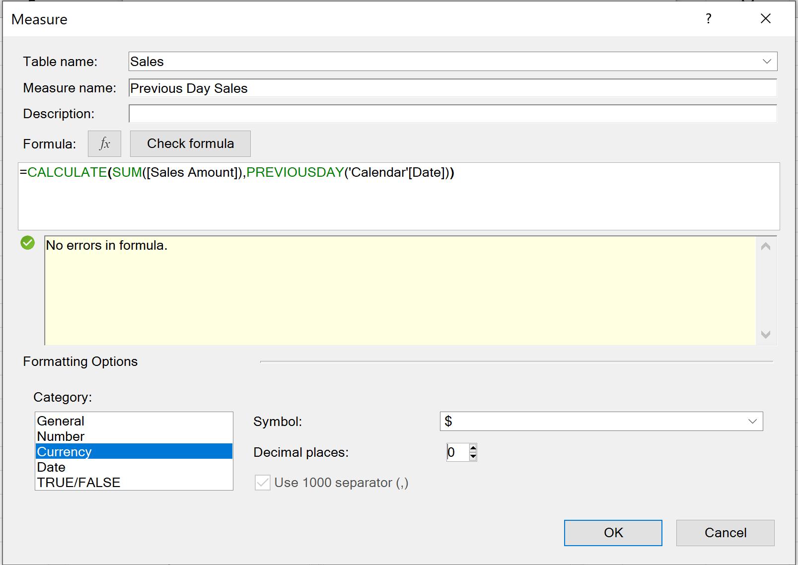
Now, we navigate to the ‘Power Pivot’ tab on the Ribbon, click Measures -> ‘New Measure…’, in order to create a ‘Previous Day Sales’ measure:

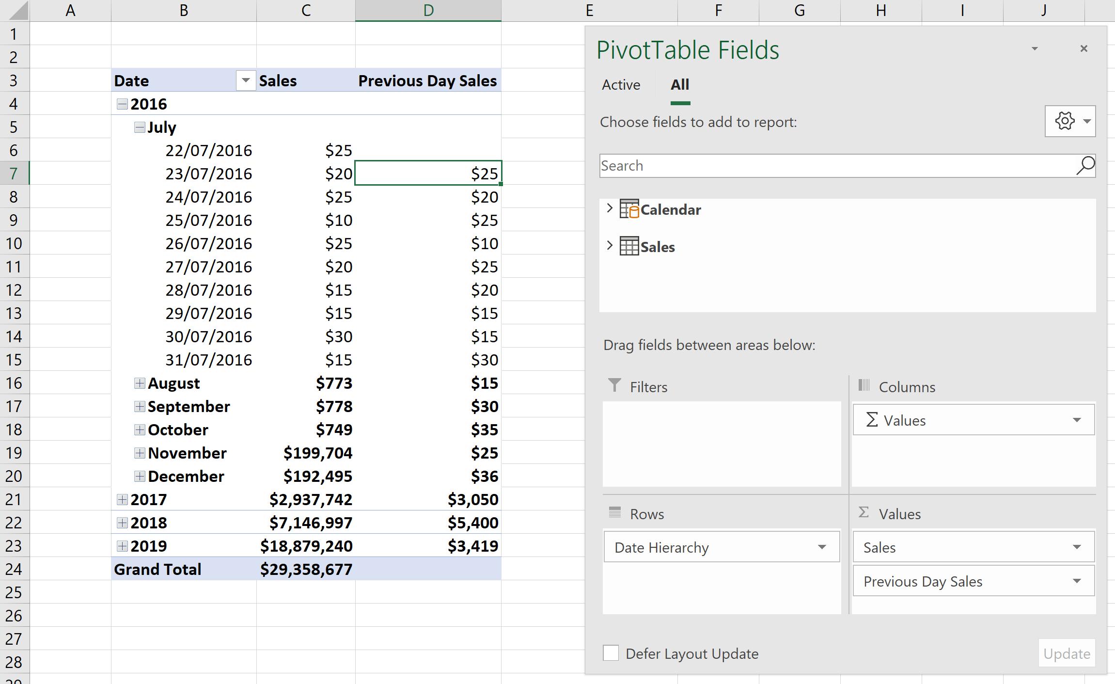
We click OK and come back to our PivotTable and drag the ‘Previous Day Sales’ to the Values field. We now have a ‘Previous Day Sales’ column to compare with Sales. Please note that the Subtotal of the months in Sales column sums all sales in a particular month, while in the ‘Previous Day Sales’ column it shows the sales of the last previous date (e.g. $15 in in August 2016 is actually sales of date 31/7/2016):

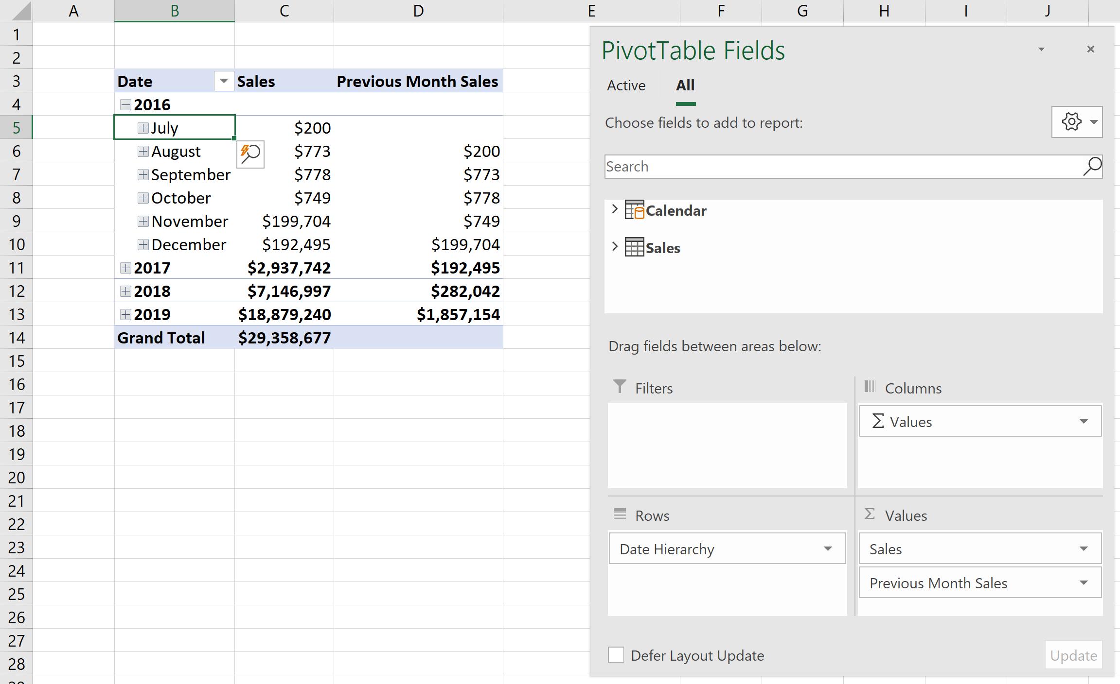
Similarly, we will create measure for ‘Previous Month Sales’:

The ‘Previous Month Sales’ reflects sales of the previous month: 

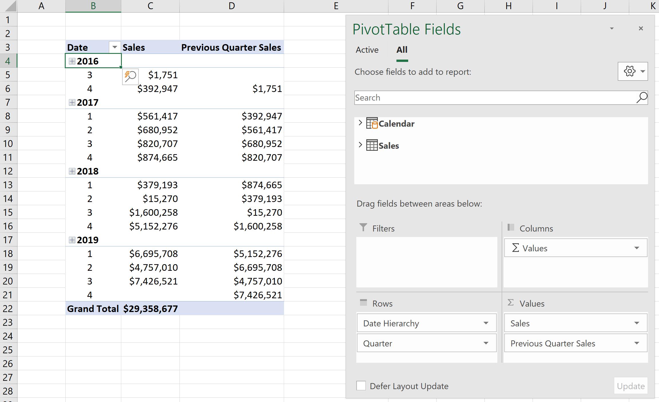
For ‘Previous Quarter Sales’:

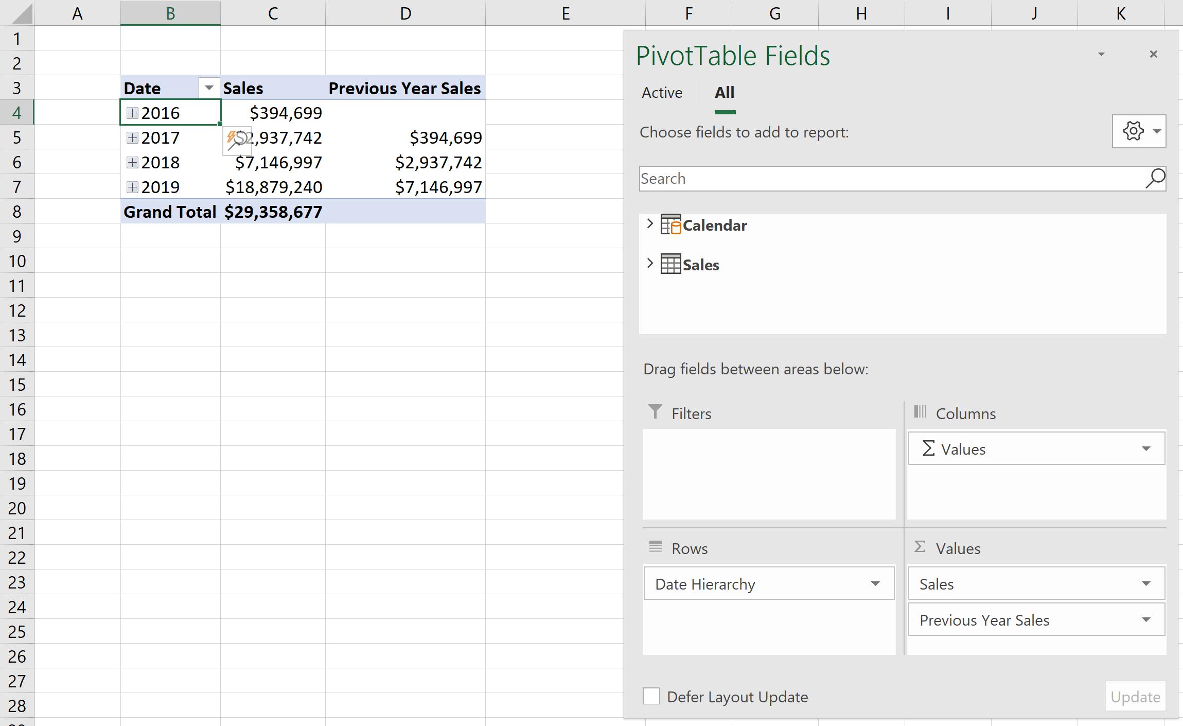
And for ‘Previous Year Sales’:

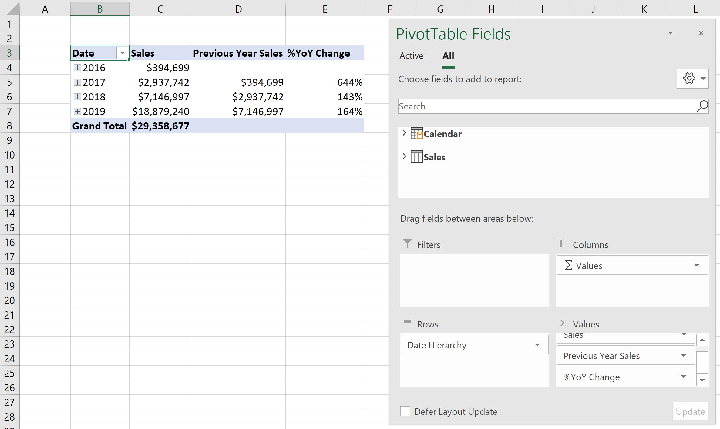
To take a step further, we want to see the sales growth by creating a measure ‘%YoY Change’:

That’s it for this week!


Stay tuned for our next post on Power Pivot in the Blog section. In the meantime, please remember we have training in Power Pivot which you can find out more about >here. If you wish to catch up on past articles in the meantime, you can find all of our Past Power Pivot blogs here.