Power Pivot Principles: Introducing the SWITCH Function

Welcome back to our Power Pivot blog. Today, we introduce the SWITCH function.

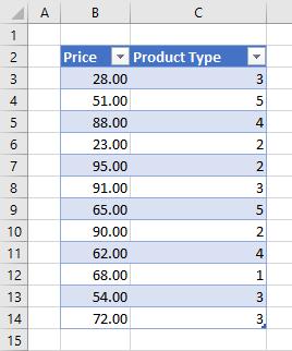
While working with data, it would be reasonable to assume that we have had add data to a data table based on values in a single column. Let’s jump into our example, we will look at the following data:

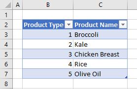
We have a simple table with the product ‘Price’ and ‘Product Type’, however numbers do not really tell us much about the product type. This is why we like to match these numbers to their corresponding text values. In this case:

Great, how do we bring in the ‘Product Name’ field into the first table?

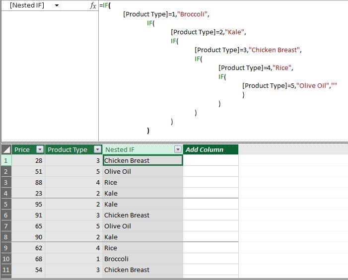
One solution would be to use a nested IF formula to create a calculated column:

Rather nasty isn’t it?  Nasty sometimes works: 

Thinking down the line, what if we had to add more product types to our table and consequently more IFs to our nested IF formula?

There is an alternative for a scenario like this, introducing the SWITCH function.  The SWITCH function requires the following syntax to operate:

The arguments for SWITCH are as follows:

• the <expression> term requires a single scalar value that can be evaluated multiple times for each row or column
• the <value> term is the constant value that will be used to match the results of the <expression>
• the <result> is the scalar value that will be returned in the column if the <value> matches the <expression>
• the <else> term is the expression that will be returned in the column when no matches are found. 

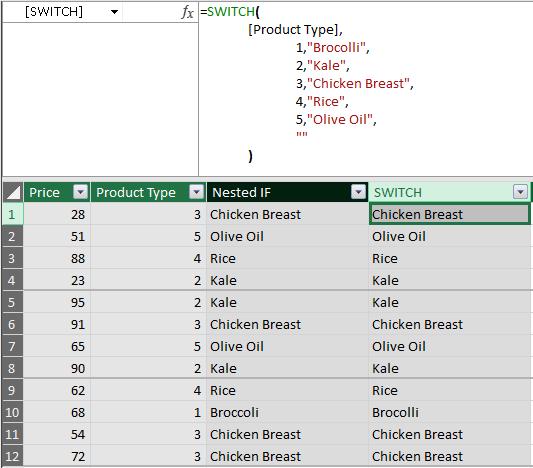
We can write the following DAX code to create a calculated column:

There we have it a DAX formula that is much easier to understand and easily expandable. 

That’s it for this week, tune in next week for more Power Pivot!  Until then, happy pivoting!

Stay tuned for our next post on Power Pivot in the Blog section.  In the meantime, please remember we have training in Power Pivot which you can find out more about here.  If you wish to catch up on past articles in the meantime, you can find all of our Past Power Pivot blogs here.