
Power Pivot Principles: Understanding Functions for Parent-Child Hierarchies in DAX – Part 4
24 December 2019
Welcome back to the Power Pivot Principles blog. This week, we are going to look at an example of applying functions for parent-child hierarchies in a business case.
Parent-child hierarchies can be used in many business scenarios. For example, most profit and loss statements have a native parent-child hierarchy for representing the chart of accounts. Although it is not the native representation in the data source, a parent-child hierarchy can be applied to show an alternative custom grouping of original accounts, such as Balance Sheet reclassification. It is also useful for the analysis of Bill of Materials (BOM) in inventory management. A list of components of a product is usually a native parent-child hierarchy since each component has other subcomponents, with different levels of depth in different branches of the hierarchy. Hierarchies can map this relationship in a clear and logic tree structure.
Suppose we have a staff table containing Staff Key and name of Leader, with a Parent Key column that define the parent level of each staff. Also, a data table containing the sales information for each staff as shown below:


Table HR has a one-to-many relationship with the table Invoice:

After importing both tables into Power Pivot, we create a calculated column Path by using the PATH function:
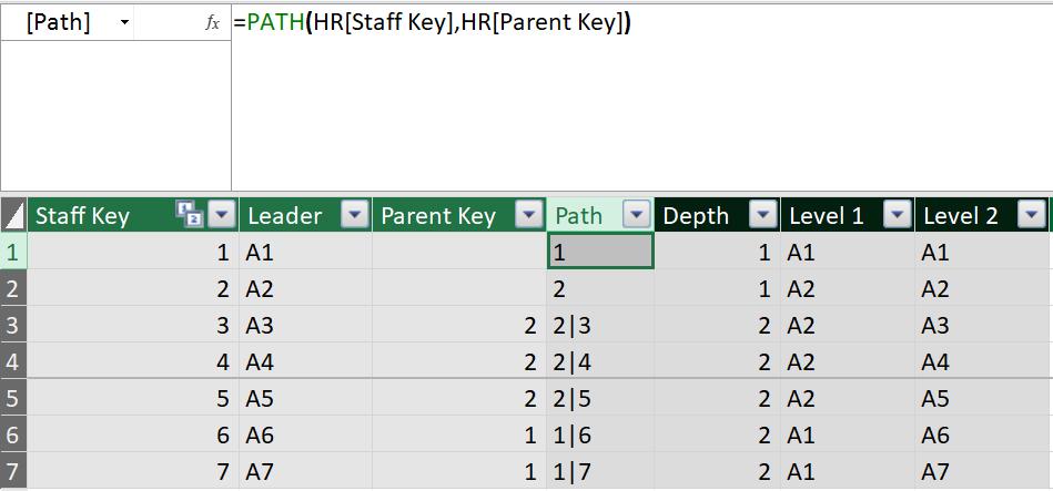
The PATH function returns the hierarchy based on the Staff Key number and Parent Key number. Then, we create another column Depth by using PATHLENGTH function:
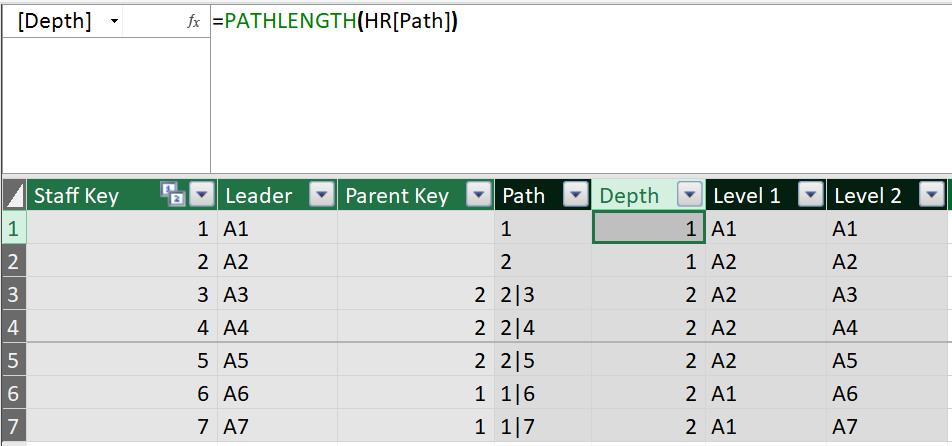
PATHLENGTH returns the level of the hierarchy based on the results obtained from PATH. In this case, the maximum level of length is two since there are only two unique values in Parent Key.
Next step, we create two additional calculated columns Level 1 and Level 2 respectively:
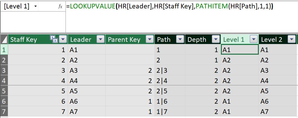
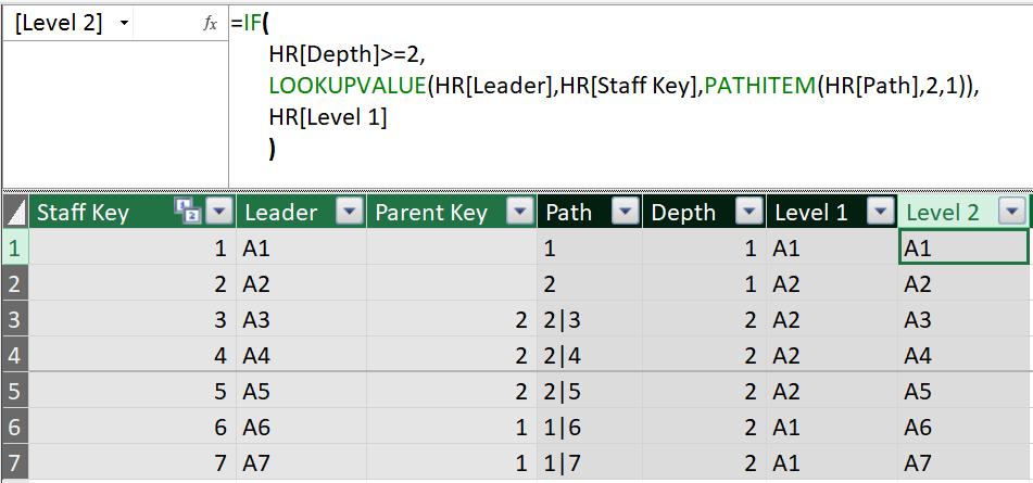
For Level 1, we use LOOKUPVALUE function to define the criteria for staff number and return the name in column Leader. Similar logic is applied in the Level 2 calculation. The only difference is that we define the Depth >= 2 as the selection criteria for the name to be returned since we only want to list the second level staff.
Finally, we create a PivotTable based on the relationships and calculated column created. The result would be:
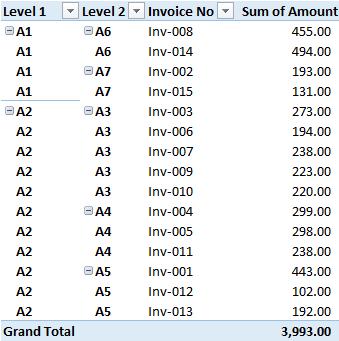
The table above shows the total sales amounts for different invoice numbers per different staff levels.
That’s it for this week!
Stay tuned for our next post on Power Pivot in the Blog section. In the meantime, please remember we have training in Power Pivot which you can find out more about here. If you wish to catch up on past articles in the meantime, you can find all of our Past Power Pivot blogs here.