Power Pivot Principles: Variables and Disconnected Tables in Power Pivot

Welcome back to our Power Pivot blog.  Today, we revisit using Variables and Disconnected tables, this time in Power Pivot

Last week we detailed a method using variables and disconnected tables to create a dynamic toggle to display our data in Power BI (see Power Pivot Principles: Variables and Disconnected Tables in Power BI for more details).

We are going to revisit the dynamic toggle this week and construct it with Power Pivot in Excel!  As detailed in last week’s blog, the SELECTEDVALUE function is not in Power Pivot’s DAX library.  Therefore, we have to use a combination of functions to replicate the formula in Power Pivot.

To replicate the SELECTEDVALUE result we have to use a combination of the IF, HASONEVALUE and VALUES functions in the following manner:

The HASONEVALUE function will return with TRUE when the column name has been filtered down to one distinct value, otherwise it will return with FALSE.  This is a useful function when you want a different formula for subtotals and totals, for example.

The VALUES function returns with a single text value from the ‘Division Types’ column.  This function will not function properly if the column is not filtered down to a single value.  Therefore, we need to employ the use of the HASONEVALUE function and the IF function as an error trap for the measure. 

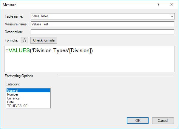
If we create the following measure with just the VALUES function: 

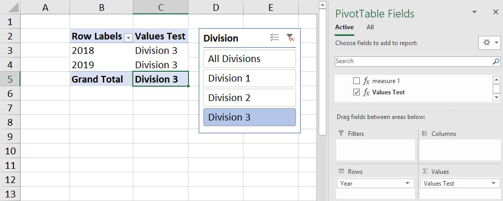
The PivotTable will return with the single column value from ‘Division Type’:

Working in Excel, the VALUES function will return the following error message when there is no filter on the slicer:

Moving on to the Power Pivot solution, we replace the SELECTEDVALUE segment of code from our previous blog,

with the first piece of code detailed above to yield:

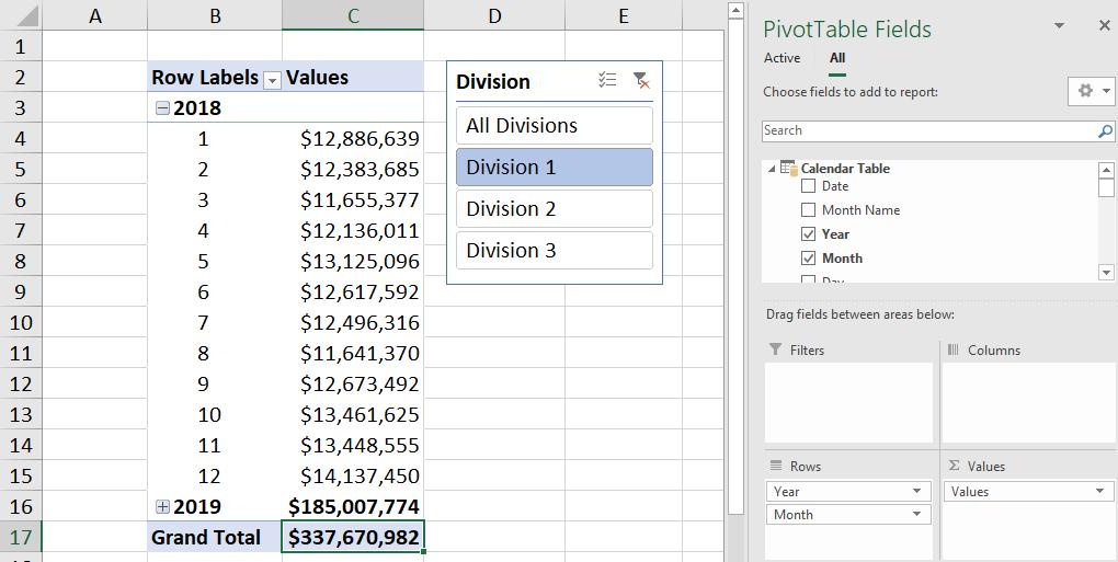
Assuming that we have imported all of the data into our data model and created the relevant relationships between our tables and slicers, we can construct the following PivotTable:

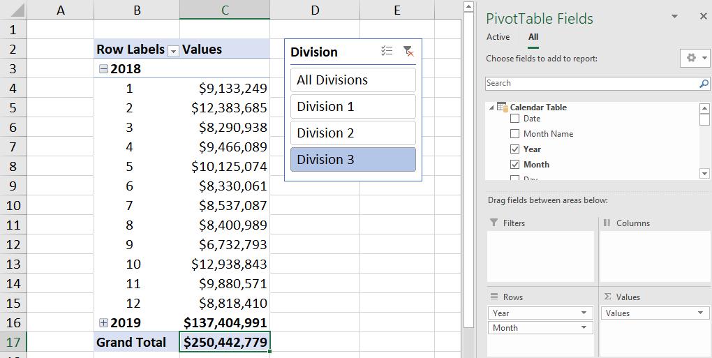
Changing the selection on the slicer will yield:

We can now dynamically toggle between divisions in our PivotTable in Excel!

That’s it for this week, happy pivoting!

Stay tuned for our next post on Power Pivot in the Blog section. In the meantime, please remember we have training in Power Pivot which you can find out more about here. If you wish to catch up on past articles in the meantime, you can find all of our Past Power Pivot blogs here.