Power Pivot Principles: When the CALCULATE Function Misbehaves.
8 January 2019
Welcome back to our Power Pivot blog. Today, we discuss how to stop the CALCULATE function from overwriting row filters.
Let’s say we wish to create a measure to calculate the total sales of all products classified as Product Category 2.
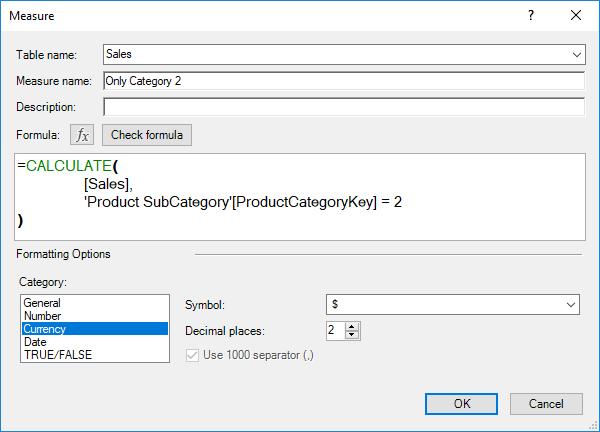
Let’s try this with the CALCULATE function:
=CALCULATE(
[Sales],
'Product SubCategory'[ProductCategoryKey] = 2
)

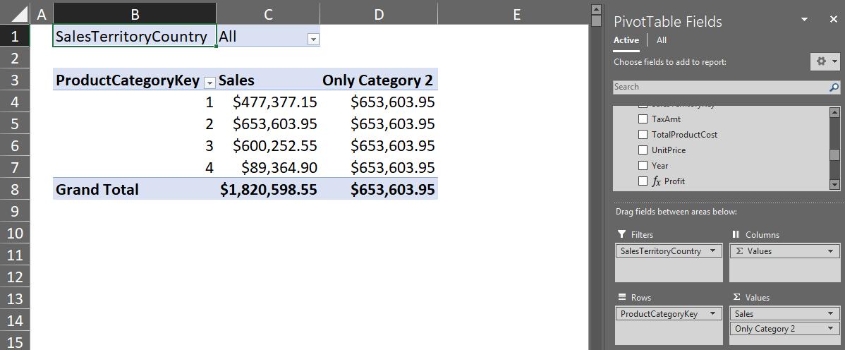
The Only Category 2 measure yields:

In this case the CALCULATE measure overrides the row context in cells C4:C7 to be ProductCategoryKey = 2 instead of their respective values (i.e. 1, 2, 3 or 4).
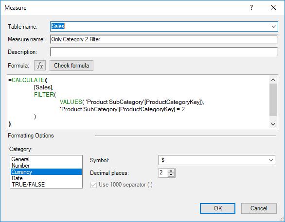
Let’s try adding the VALUES function into a measure:
=CALCULATE(
[Sales],
FILTER(
VALUES( 'Product SubCategory'[ProductCategoryKey]),
'Product SubCategory'[ProductCategoryKey] = 2
)
)

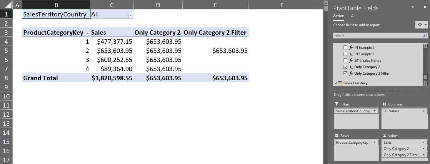
This measure yields:

Voilà! Using the VALUES function we have managed to alter the CALCULATE function’s behaviour and stop it from overriding the row context values. Our data no longer has the same values for each Product Category!
That’s it for this week, happy pivoting!
Stay tuned for our next post on Power Pivot in the Blog section. In the meantime, please remember we have training in Power Pivot which you can find out more about here. If you wish to catch up on past articles in the meantime, you can find all of our Past Power Pivot blogs here.

