
Power Query: Flexible Appending – Part 3
16 November 2022
Welcome to our Power Query blog. This week, I am continuing to combine data from a folder and to use a translation table to create column names.
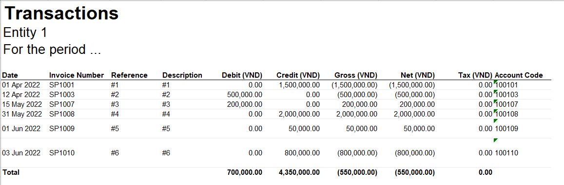
As previously, I have three [3] Excel workbooks, each with accounting data. The first file looks like this:
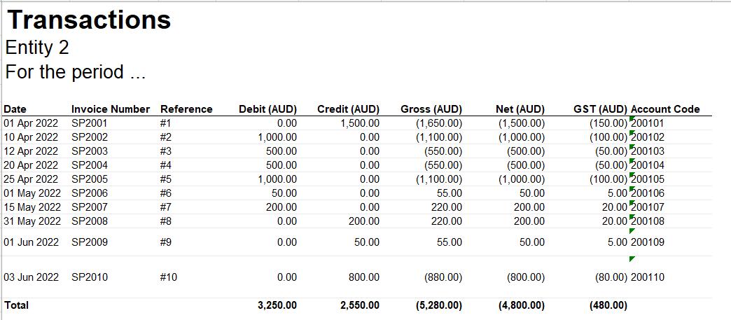
The second file looks like this:
The final file looks like this:
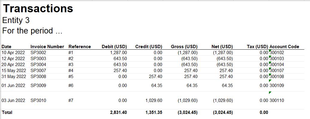
There are clearly some differences between the files. The column headings vary by country, and the first file has an extra column.
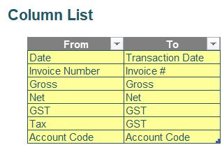
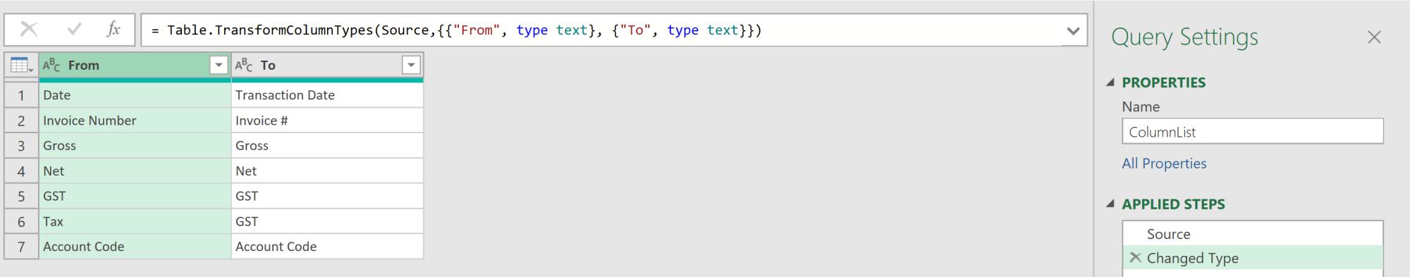
My goal is to get this data into the same table. For the purposes of this example, I am not required to convert the figures to the same currency. However, I do need to allow for more files appearing from other countries. The files are held in one folder. I have a translation table Column List in a separate Excel workbook (shown below) to help me determine the column names in the final table. No other columns are required apart from the ‘entity’ name (e.g. ‘Entity 1’).
In Part 1, I created a query ColumnList:
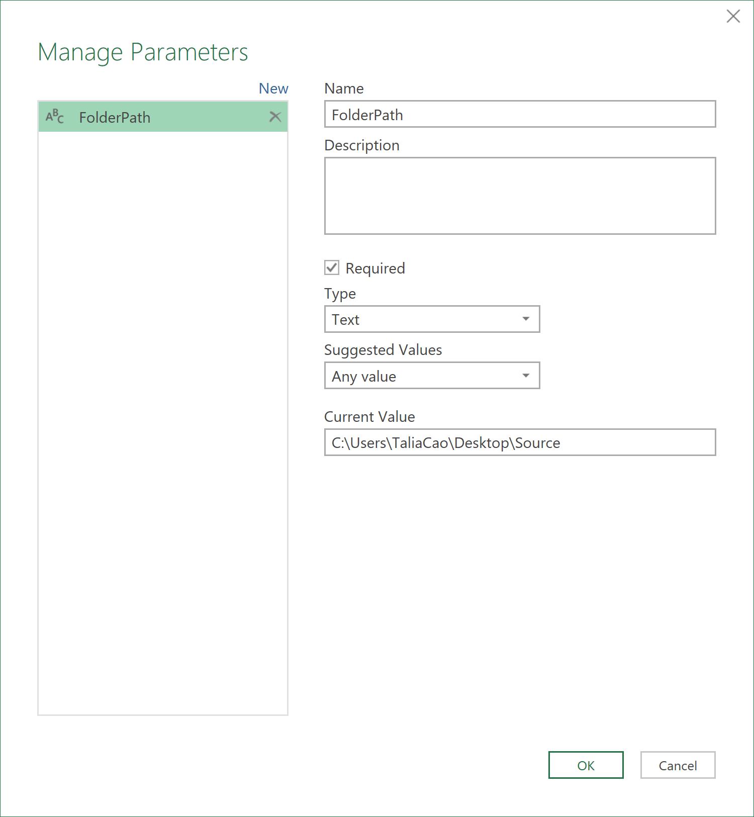
I also created a parameter called FolderPath. The ‘Current Value’ of the parameter is the folder path containing the files that I am going to append.
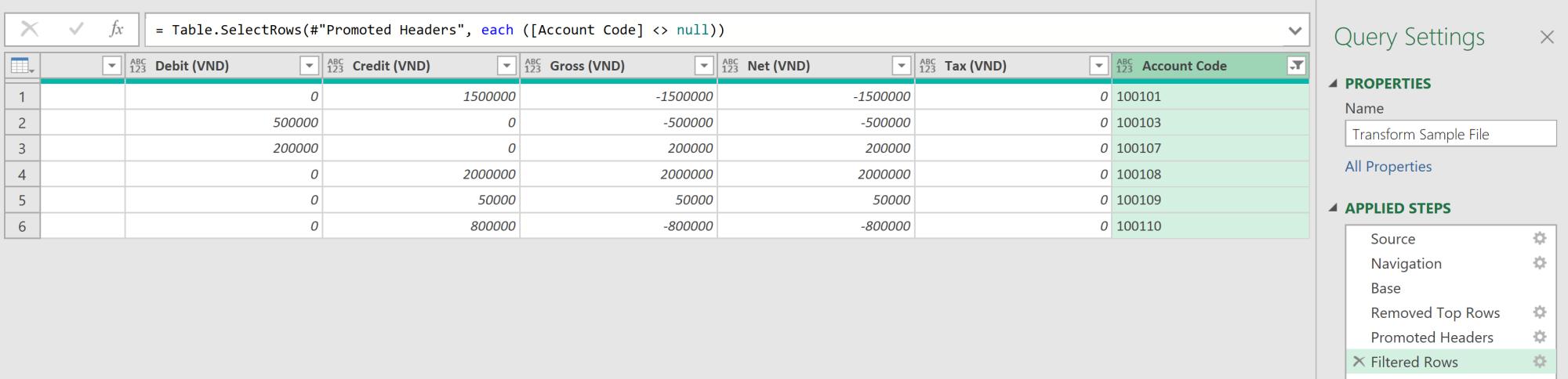
I also created and transformed a query Transform Sample File, which will act as the basis for the transformation that I need to apply to each Excel workbook in the folder.
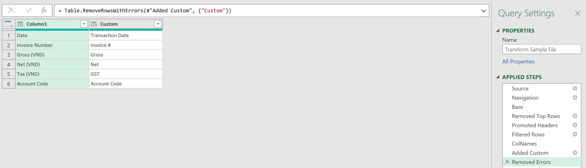
Last time, I created a table of original and standardised column names for the sample file.
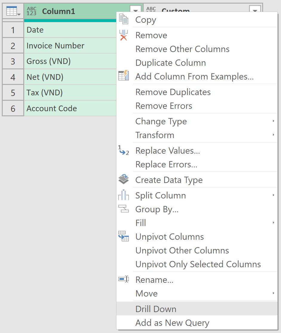
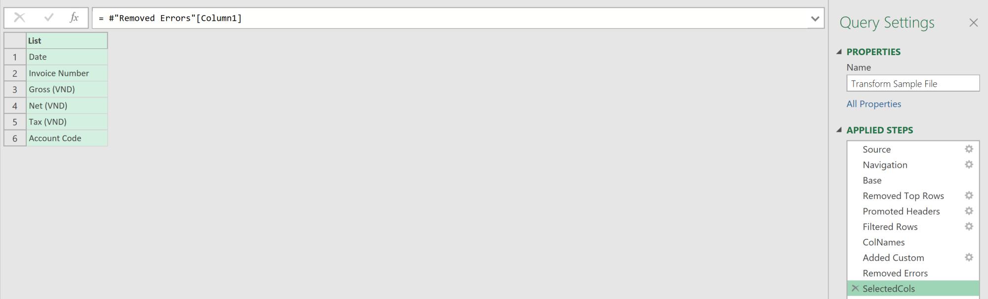
This week, I will complete the example by applying the list to each of the extracted Excel sheets. I need to convert Column1 to a list by right clicking the column header and selecting ‘Drill Down’. I name the new step ‘SelectedCols’.
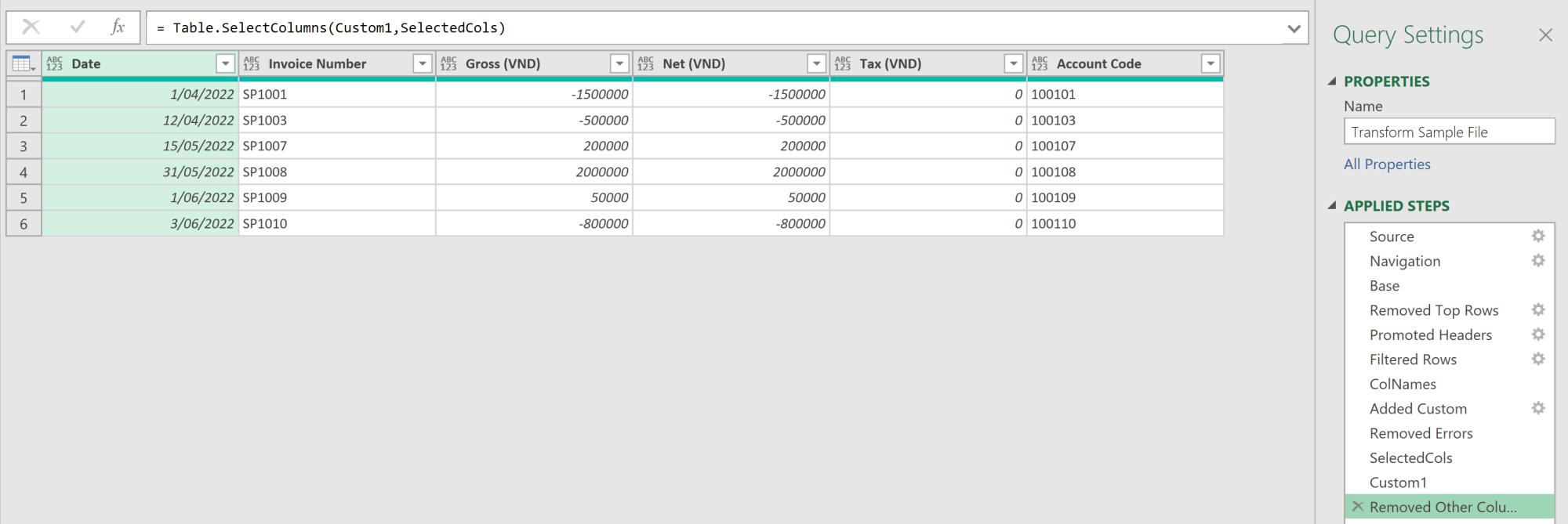
Then, I add a new blank step and refer it back to the ‘Filtered Rows’ step. I select a few columns to keep (it doesn’t matter which, as I am getting the M ‘framework’ for the step) and apply ‘Remove Other Columns’ to have Power Query produce the M code below for me.
= Table.SelectColumns(Custom1,{"Date", "Invoice Number", "Gross (VND)", "Net (VND)", "Tax (VND)", "Account Code"})
I can replace the hardcoded column list with SelectedCols:
= Table.SelectColumns(Custom1,SelectedCols)
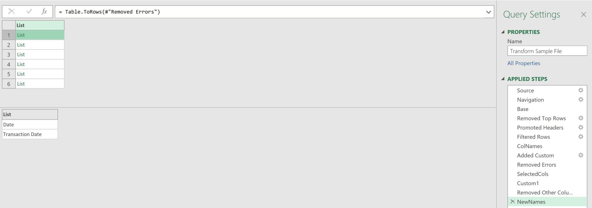
Finally, I need to rename the columns. I create a blank step referring to ‘Removed Errors’ step and edit the step to use a Table.ToRows function to convert the table into a list of lists.
= Table.ToRows(#"Removed Errors")
Each child list contains an original name and its new standardised name. I rename this step ‘NewNames’.
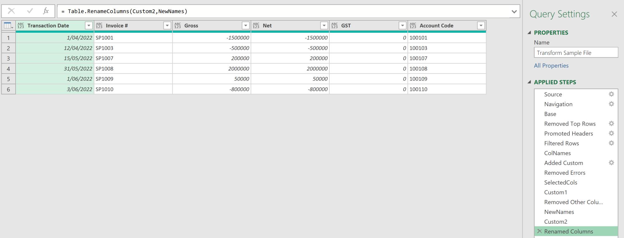
I then create a blank step referring to the ‘Removed Other Columns’ step and rename a few columns to get autogenerated M code in the same way as I did for the ‘SelectedCols’ step. The hardcoded part can then be replaced by NewNames:
= Table.RenameColumns(#"Removed Other Columns",NewNames)
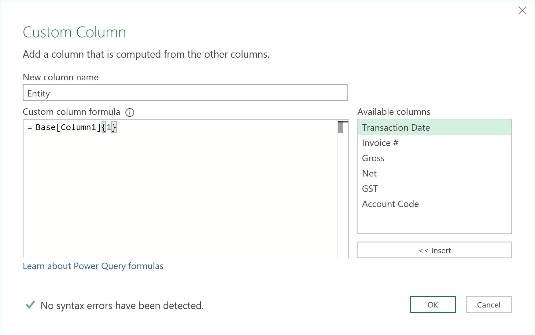
Finally, I add a custom column Entity by using the following M code:
= Base[Column1]{1}
This refers to Column1and the second row of the ‘Base’ step where entity name is located (note that Power Query begins counts at zero [0]).
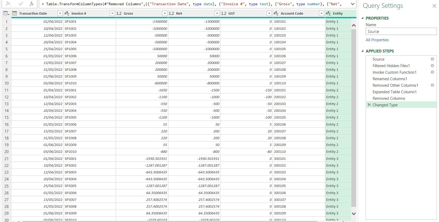
The Transform Sample File query is complete. Let’s now return to the main Source query.
There is an error in the automatically generated ‘Changed Type’ step as the Transactions column no longer exists. I can safely delete the ‘Changed Type’ step. Then, I right-click and remove the Source.Name column. Finally, I change the column data types from ‘Any’ to the appropriate type for each column.
The data is ready to ‘Close & Load’. However, I could have also made the ‘Changed Type’ step dynamic too, rather than selecting the appropriate type manually. I’ll look at this next time…
Come back next time for more ways to use Power Query!