Power Query: Pivot the Blanks

Welcome to our Power Query blog. This week, I look at another way to remove blank rows and columns which will allow me to keep column names.

The scenario is familiar, a huge Excel table comes in with lots of columns and rows, but in some cases a column or row is empty and it needs to be condensed. This may be easy to do by hand for small tables, but for large data sets it would be nice to be able to do this automatically at the press of a button.

This time I am going to use the unpivot function, because it includes some functionality which is useful to me to achieve my goal – empty cells are ignored.

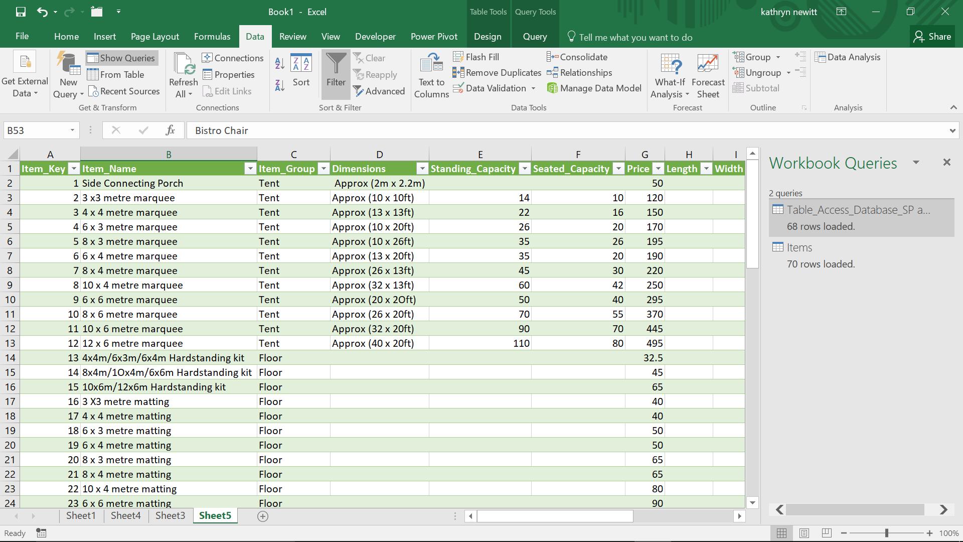
I start off with my ‘Items’ table in my workbook, and this time I include column names:

In the ‘Data’ tab, in the ‘Get and Transform’ section, I create a query ‘From Table’:

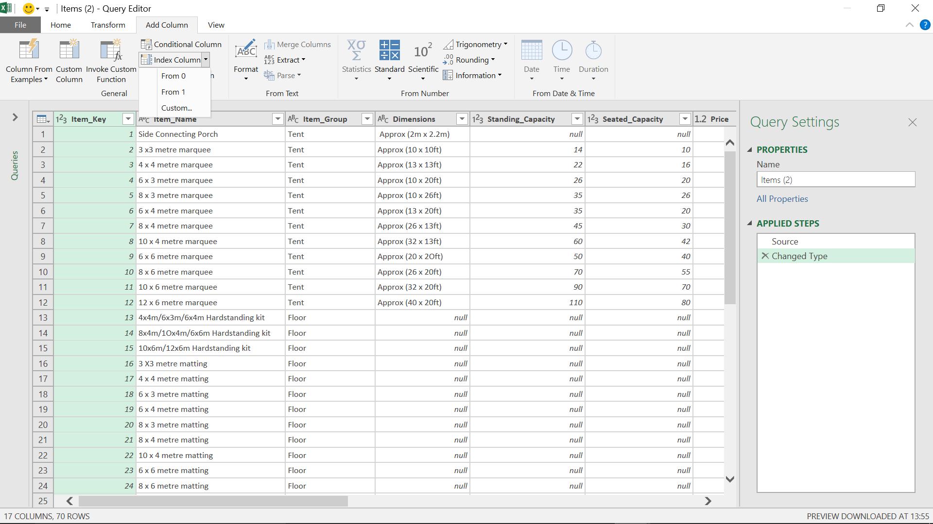
My first step will be to create an Index column – I can do this in the ‘Add Column’ tab. It doesn’t matter where my index starts from; I just need a column that will remain constant through my transformations.

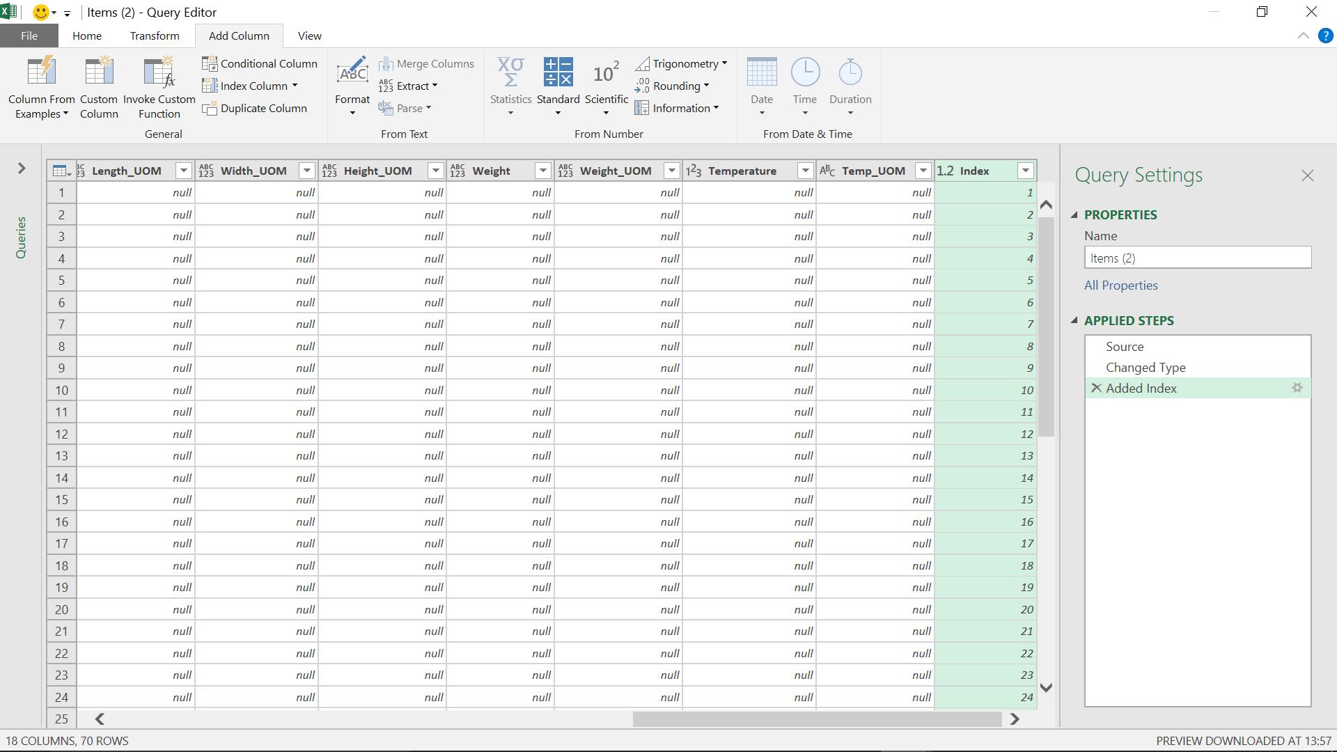
Having created my column, I right click on it and choose to ‘Unpivot Other Columns’.

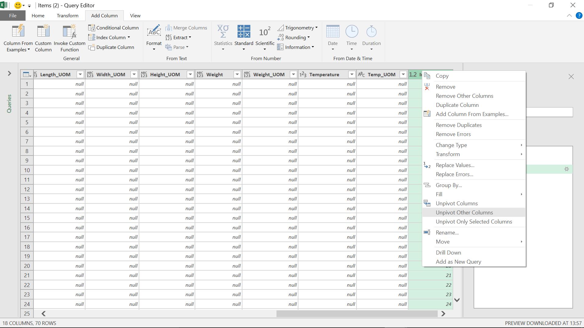
The columns will be unpivoted and my 18 columns and 70 rows are about to change…

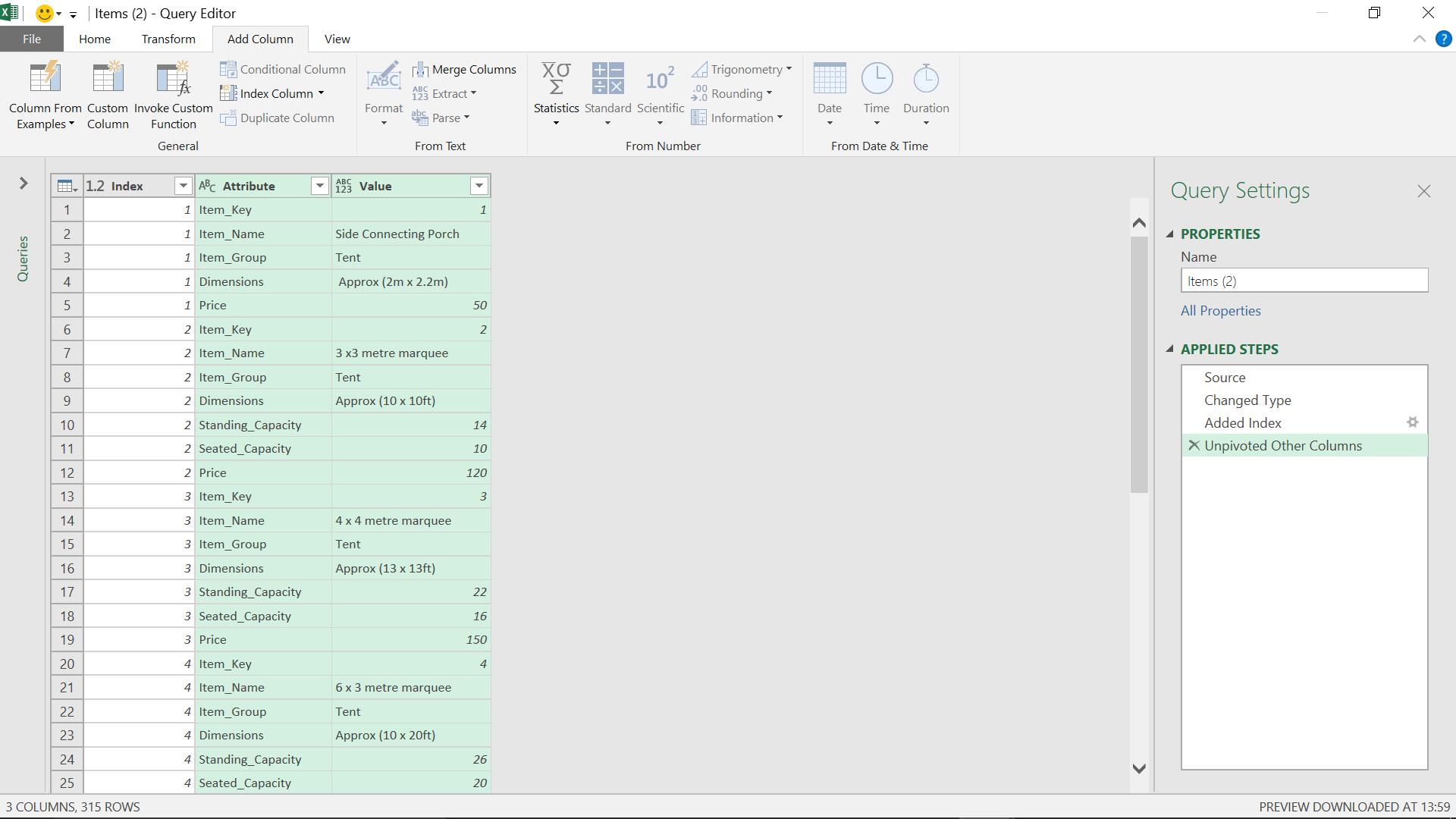
My data is now made up of Attribute and Value. Now I need to pivot my data again, so I select my Attribute column and choose ‘Pivot Column’ from the ‘Transform’ tab.

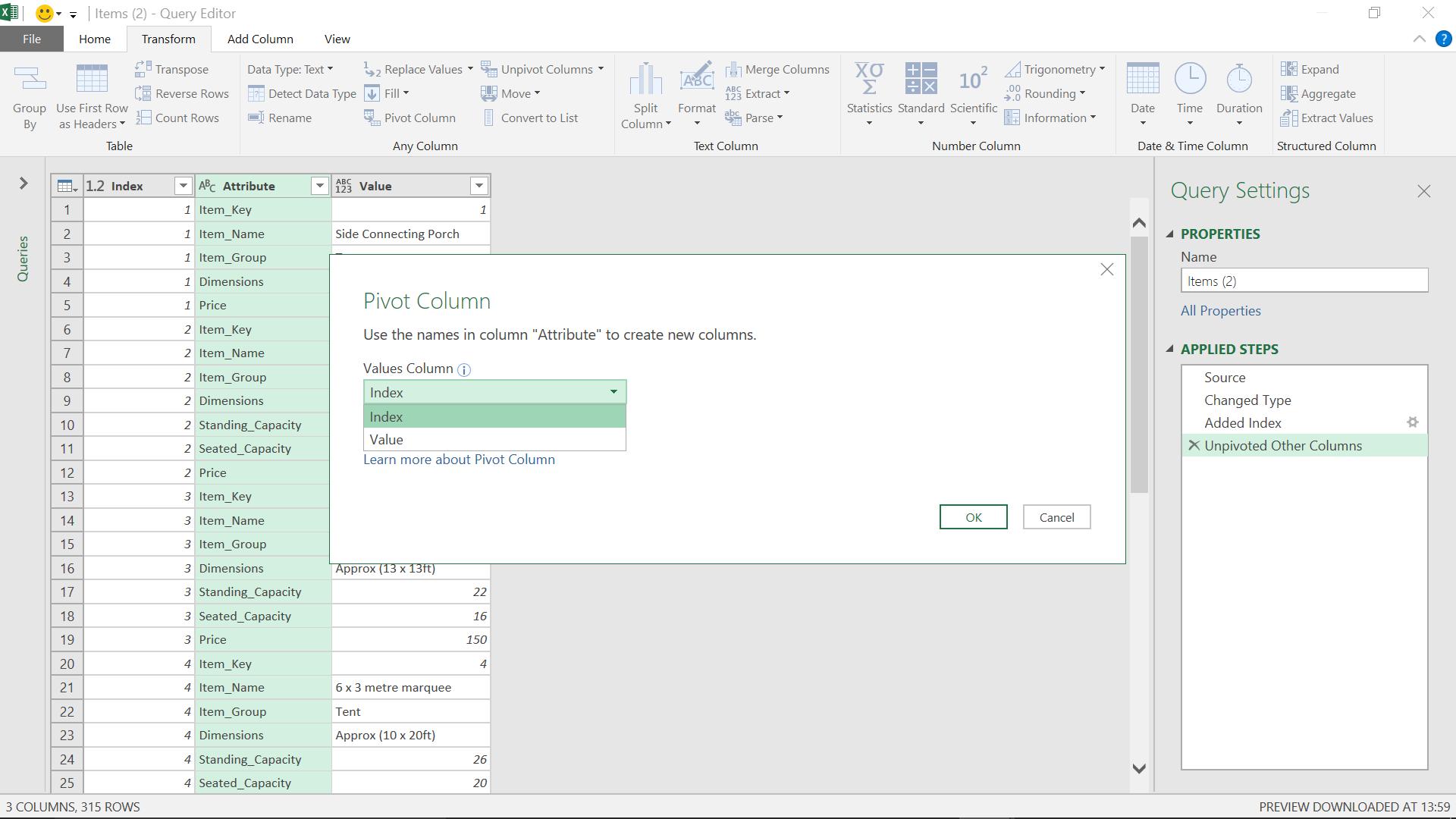
I am prompted to choose a ‘Values Column’ for the columns I am going to create using my Attributes column. I choose Value.

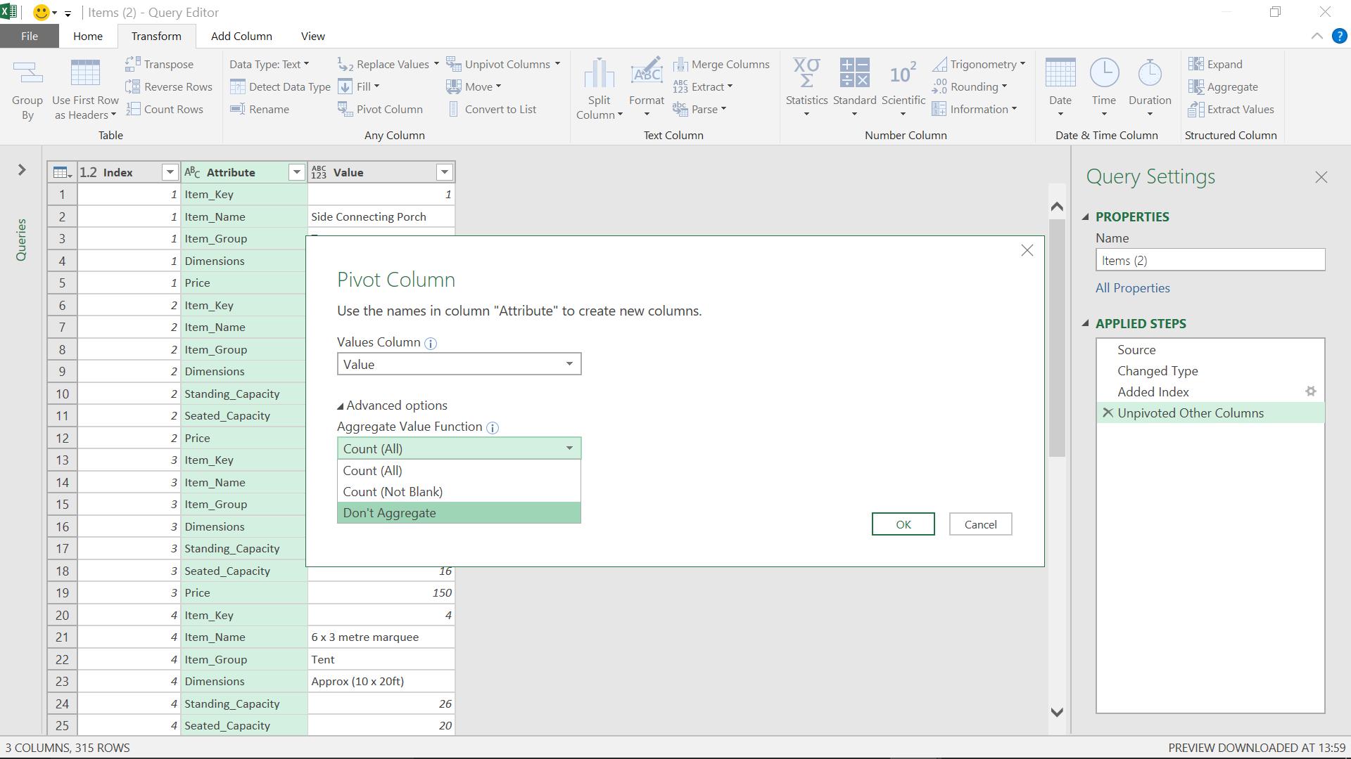
As I don’t want to manipulate any of my data I also go into the advanced options to make sure that I choose ‘Don’t Aggregate’. I then click ‘OK’ to pivot my data.

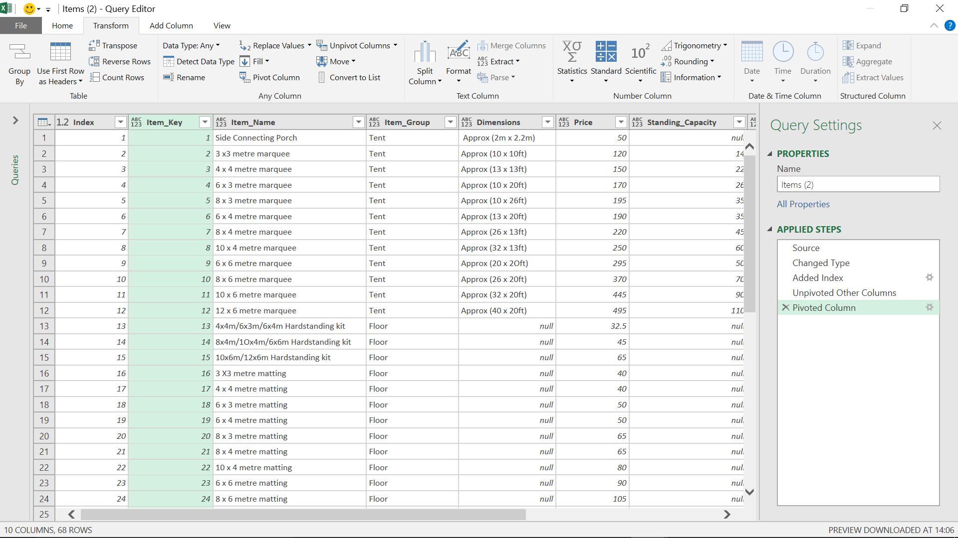
All my blank rows and columns have been removed! I just need to delete my index column and my data is ready to be loaded. All without losing my column headings too (although I do note headers could have been demoted in last week’s demonstration)!

Want to read more about Power Query? A complete list of all our Power Query blogs can be found here.