Power Query: Pivotal Pivoting

Welcome to our Power Query blog. Today I look at pivoting a column.

Power Query’s ability to efficiently transform data is amply demonstrated by features which allow me to pivot (and unpivot) data at the touch of a button. I begin as usual with my data in an Excel worksheet.

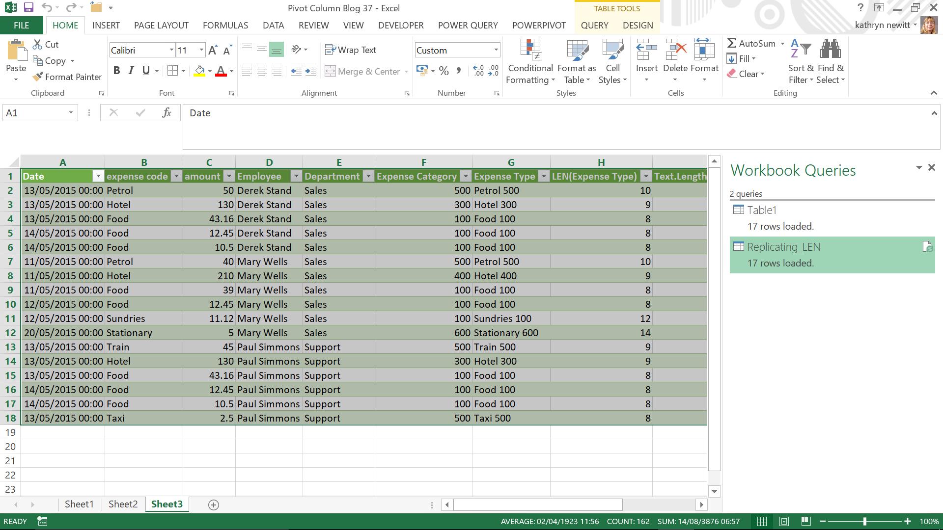
In the ‘POWER QUERY’ tab, in the ‘Excel Data’ section, I choose to extract my data ‘From Table/Range’:

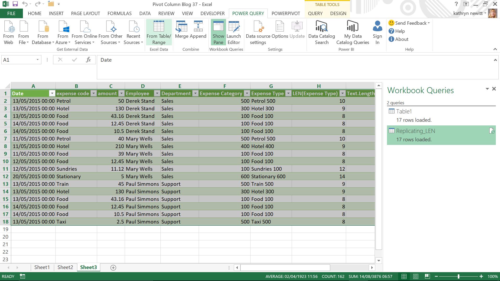
My data appears in a new query, which I have called ‘Pivot Column’. In the ‘Transform’ tab, there is a section which groups together the transformations which can be applied to ‘Any Column’. I am interested in the ‘Pivot Column’ option.

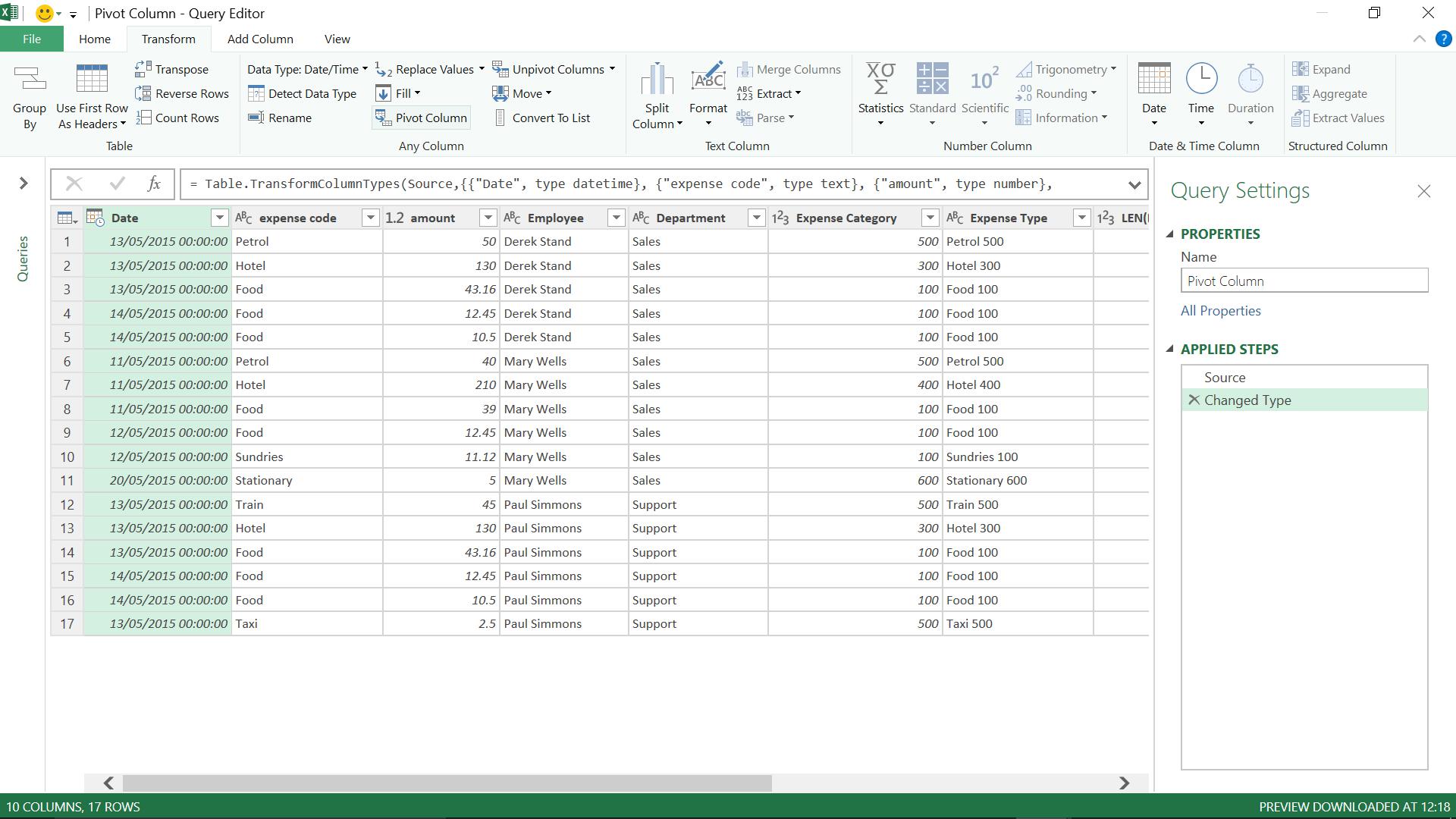
‘Pivot Column’ is available as long as I haven’t selected multiple columns.  I can either select a column before using ‘Pivot Column’ or it will assume I want to use the first column in my query.  I select expense code.

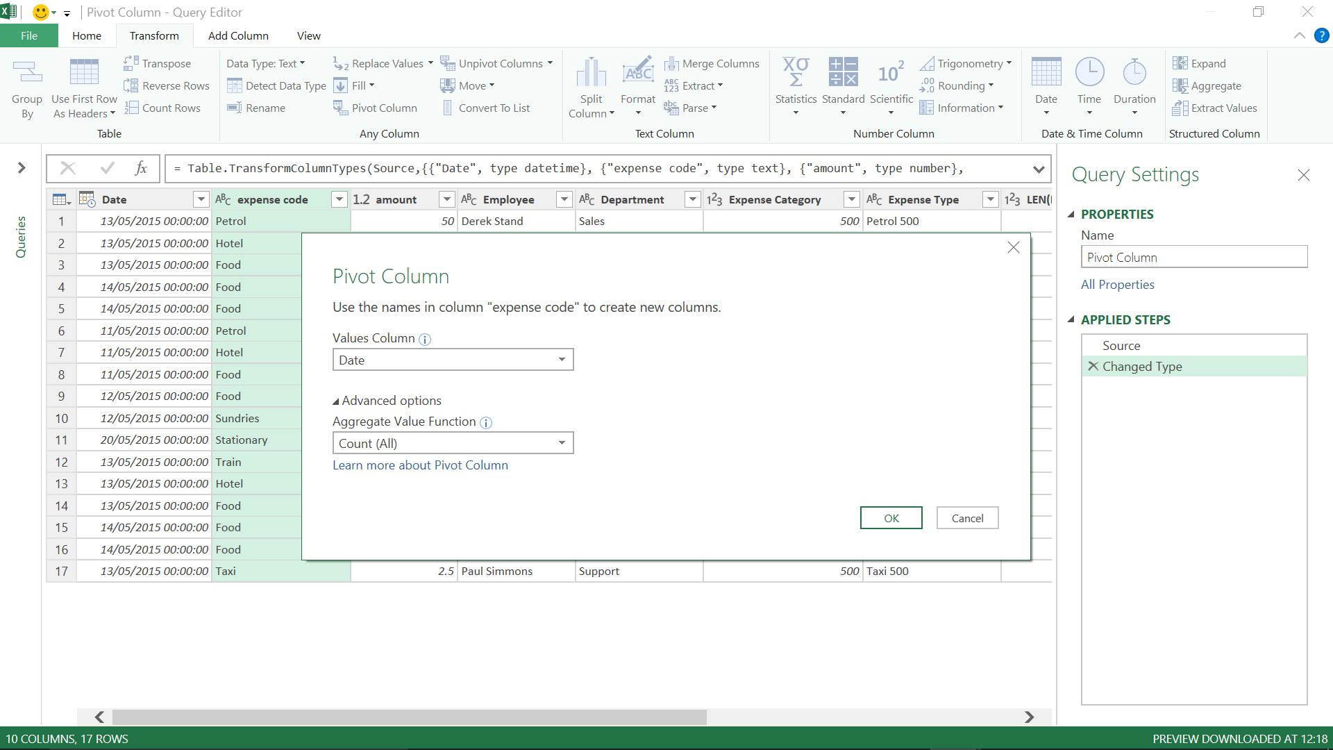
The ‘Pivot Column’ feature will remove my selected column and add columns to my table that contain an aggregate value for each unique value in that column.  This is quite a concept to describe in one sentence, and it best demonstrated by an example!

I have provided the names of the column (expense code), but I also need to specify what data will be aggregated, and the function associated with the aggregation.  The data column will also be removed from my query when the new columns are added.  I will be using the amount column as my data, which I have decided to sum viz.

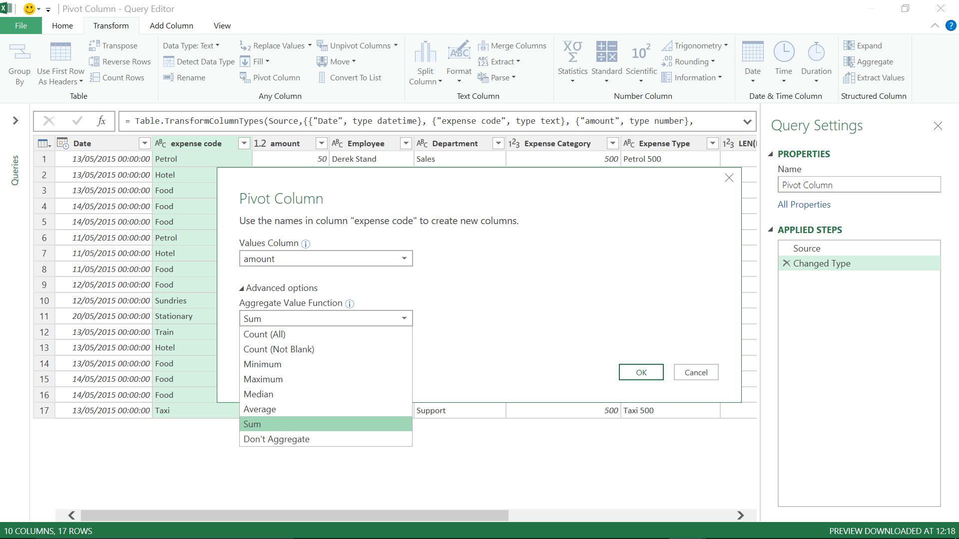
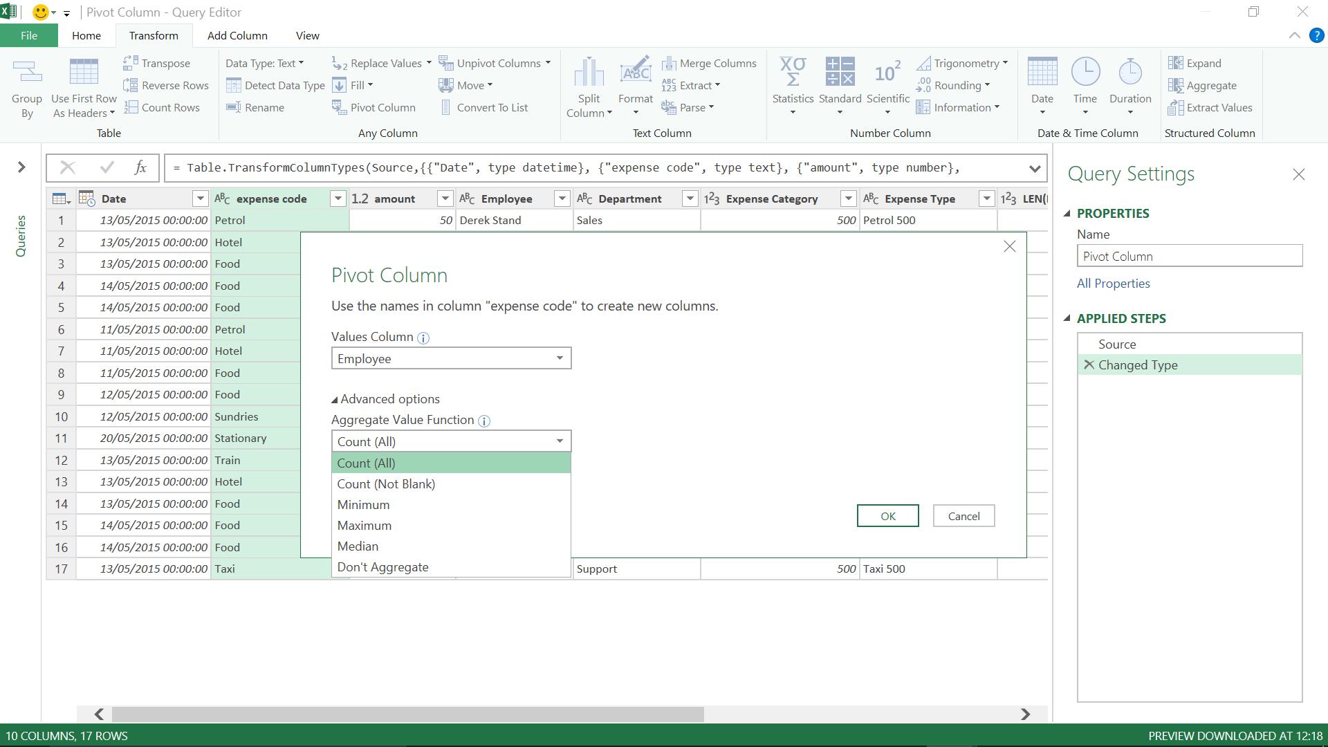
As soon as I pick amount, power query recognises that I have chosen datatype currency, and defaults to ‘Sum’. The other options for my datatype are shown above. If I had chosen a text column, then the options would be different, as shown below:

Returning to my amount column, there is also an option ‘Don’t Aggregate’.  This would return a grid which only has values when that particular expense code is populated, as shown below:

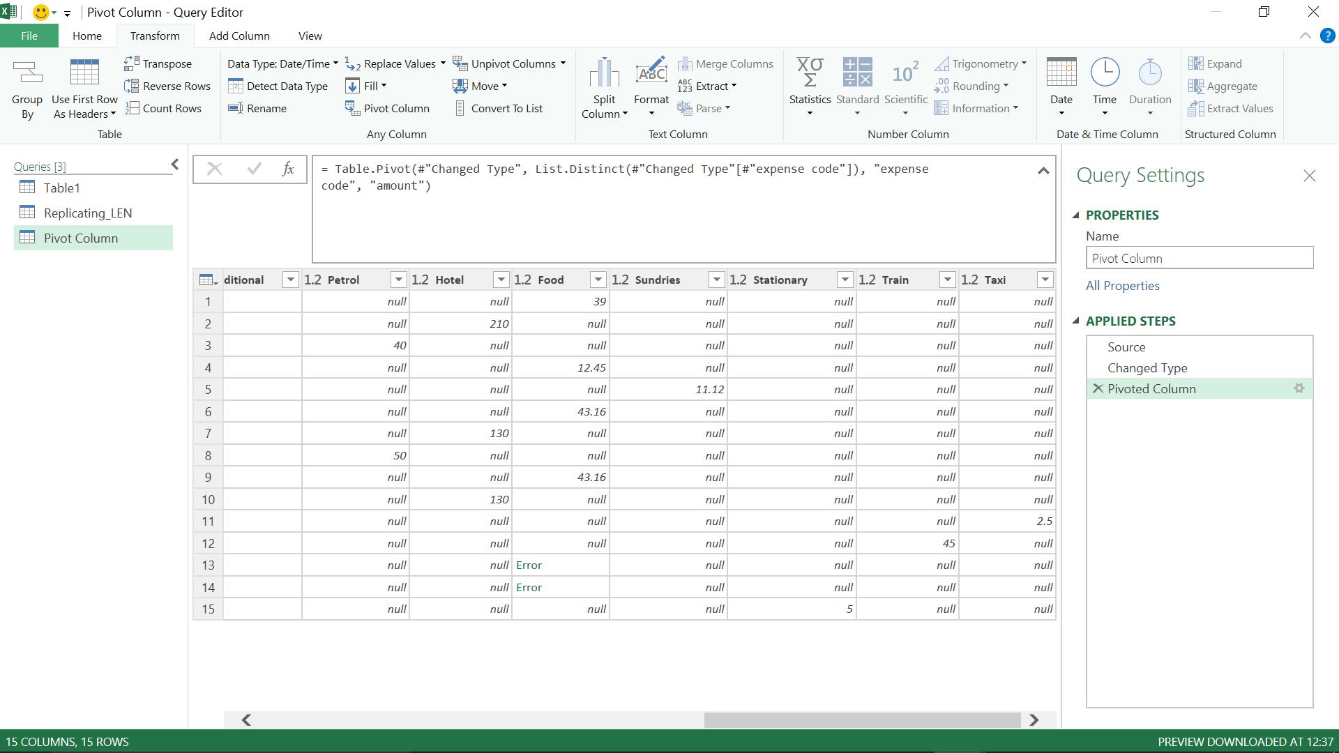
It didn’t work too well when I had two consecutive food amounts, but the other amounts are shown. I am more interested to try aggregating by using the ‘Sum’ option, so I delete this step and return to my ‘Pivot Column’ screen and try again…

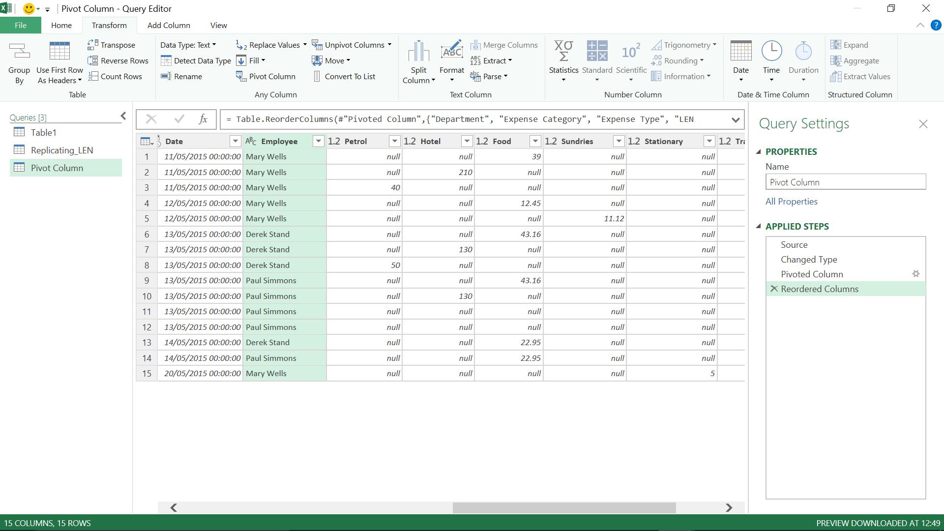
This time my data is all populated as expected. I have already reordered my columns so that I can see who incurred what expense and on what date and I can tidy it up further by removing the nulls by using the ‘Replace Values’ facility.

Having demonstrated how easy it is to pivot columns, another nice feature to show is how easy it is to unpivot them again. If I select my new columns and choose to ‘Unpivot’ them using the option from within the ‘Any Column’ section in the ‘Transform’ tab, I get this:

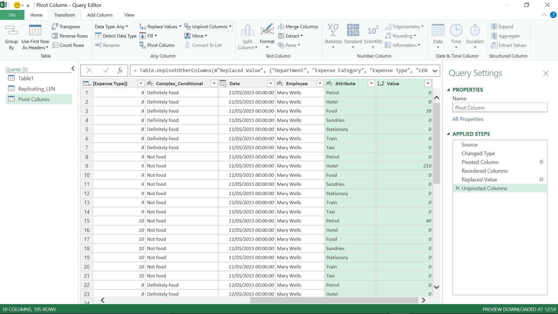
My expense code (Attribute) and my amount (Value) have been reinstated!

Want to read more about Power Query? A complete list of all our Power Query blogs can be found here.  Come back next time for more ways to use Power Query!