
New Functions Announced
15 November 2023
Microsoft announced three new functions and “eta reduced lambda” functions (known as “eta lambdas”) into the Excel family today. They make automating data analysis really simple – as long as you have access to all of these functions! They are rolling out on the beta channel for Excel for Windows and Excel for Mac as we write.
You can follow along with the attached Excel file as you wish (as long as you have access to these new functions / features).
Do note: SumProduct will be providing a FREE one-hour webinar on these new functions at 1pm Australian Eastern Daylight Time (AEDT) / 2am Coordinated Universal Time (UTC) on Tuesday 28 November.
You may register here.
If you are unable to watch the event live, please follow the registration
process, and the recording will be emailed
after the event has concluded.
eta Lambdas
These “eta reduced lambda” functions may sound scary, but they make the world of dynamic arrays more accessible to the inexperienced. They help make the other three functions simpler to use. Dynamic array calculations using basic aggregation functions often require syntax such as
LAMBDA(x, SUM(x))
LAMBDA(y, AVERAGE(y))
etc.
However, given x and y (above) are merely dummy variables, an “eta lambda” function simply replaces the need for this structure with the so-easy-anyone-can-understand-it syntax of
SUM
AVERAGE
etc.
Even I can do it. For example, consider the following formula in cell G17 below:
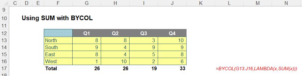
=BYCOL(G13:J16,LAMBDA(x,SUM(x)))
This sums the range G13:J16 by column using that LAMBDA(x, SUM(x)) trick. But there is no need for this anymore, viz.
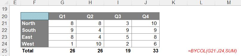
=BYCOL(G21:J24,SUM)
That’s much simpler!
Presently, the following built-in functions are available to Excel users lucky enough to get all these functions and functionalities:
- ARRAYTOTEXT
- AVERAGE
- CONCAT
- COUNT
- COUNTA
- MAX
- MEDIAN
- MIN
- MODE.SNGL
- PERCENTOF
- PRODUCT
- STDEV.P
- STDEV.S
- SUM
- VAR.P
- VAR.S
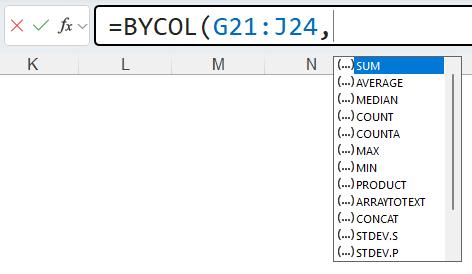
These will pop up when they may be used, but they don’t appear in alphabetical order. It’s more a ranking of what Microsoft perceives to be the most common aggregation operations:
GROUPBY
The new GROUPBY function allows you to create a summary of your data formulaically. It supports grouping along one axis and aggregating the associated values. For instance, if you had a table of sales data, you might generate a summary of sales by year, or by salesperson, or by category, or by…
In essence, it allows you to group, aggregate, sort and filter data based upon the fields you specify.
The syntax of the GROUPBY function is given by:
GROUPBY(row_fields, values, function, [field_headers], [total_depth], [sort_order], [filter_array])
It has the following arguments:
- row_fields: this is required, and represents a column-oriented array or range that contains the values which are used to group rows and generate row headers. The array or range may contain multiple columns. If so, the output will have multiple row group levels
- values: this is also required, and denotes a column-oriented array or range of the data to aggregate. The array or range may contain multiple columns. If so, the output will have multiple aggregations
- function: also required, this is an explicit or eta reduced lambda (e.g. SUM, PERCENTOF, AVERAGE, COUNT) that is used to aggregate values. A vector of lambdas may be provided. If so, the output will have multiple aggregations. The orientation of the vector will determine whether they are laid out row- or column-wise
- field_headers: this and
the remaining arguments are all optional.
This represents a number that specifies whether the row_fields and values have headers and whether field headers should be returned in
the results. The possible values are:
- Missing: Automatic
- 0: No
- 1: Yes and don't show
- 2: No but generate
- 3: Yes and show
- total_depth: this optional
argument determines whether the row headers should contain totals. The possible values are:
- Missing: Automatic, with grand totals and, where possible, subtotals
- 0: No Totals
- 1: Grand Totals
- 2: Grand and Subtotals
- -1: Grand Totals at Top
- -2: Grand and Subtotals at Top
- sort_order: again optional, this argument denotes a number indicating how rows should be sorted. Numbers correspond with the columns in row_fields followed by the columns in values. If the number is negative, the rows are sorted in descending / reverse order. A vector of numbers may be provided when sorting based upon only row_fields
- filter_array: the final optional argument, this represents a column-oriented one-dimensional array of Boolean values [1, 0] that indicate whether the corresponding row of data should be considered. It should be noted that the length of the array must match the length of row_fields.
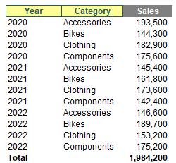
To show how GROUPBY works, we took inspiration from Microsoft’s data
table:
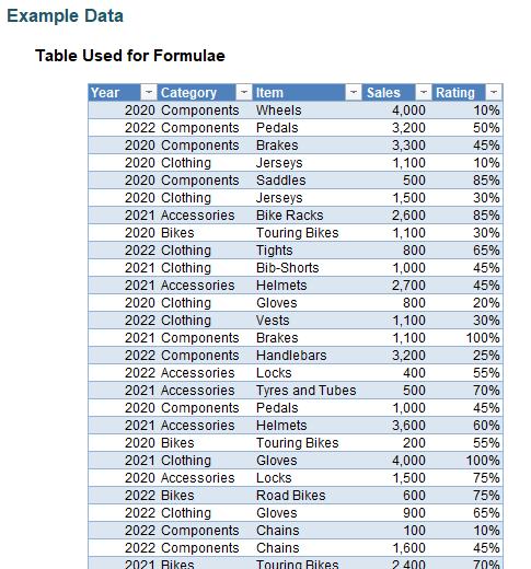
I have converted this data table into an Excel Table by selecting all the data and using Insert -> Table (CTRL + T) and calling the resultant Table tbl. Look, it’s late as I write this and I have no imagination, OK!?
I can summarise my Table very simply using the formula
=GROUPBY(tbl[Category],tbl[Sales],SUM)
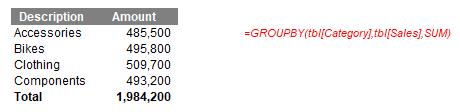
How easy is that!? Essentially, I am summing the sales (using the eta lambda SUM) by the Category field.
If you want to aggregate by more than one row_field, as stated above, this is possible. One way is to use HSTACK:
=GROUPBY(HSTACK(tbl[Year],tbl[Category]),tbl[Sales],SUM)
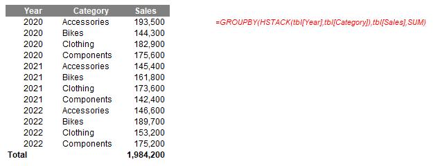
This simply combines the Year and Category fields in the tbl Table, and then sums Sales across them. However, I think I prefer the CHOOSECOLS approach:
=GROUPBY(CHOOSECOLS(tbl,1,2),tbl[Sales],SUM)
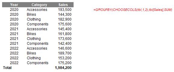
Here, the idea is that I shall SUM Sales by columns 1 (Year) and 2 (Category) of the tbl Table. This might not seem as clear as the HSTACK alternative at first glance as you have to refer to the Table to identify what the columns are. However, stick with me. Let me make the formula more complex:
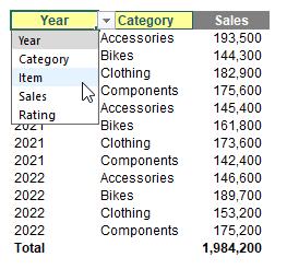
=GROUPBY(CHOOSECOLS(tbl,MATCH(F$12,tbl[#Headers],0),
MATCH(G$12,tbl[#Headers],0)),tbl[Sales],SUM)
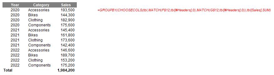
Looks horrible, yes? I have replaced the values 1 and 2 in the previous formula with
MATCH(F$12,tbl[#Headers],0)
and
MATCH(G$12,tbl[#Headers],0)
which return the positions in the Headers row of the Table tbl. Now, this may seem overkill but consider the following image:
Brilliant. I have changed the background colour of the first two headers to yellow. Well no, it’s a little more than that. I have used data validation dropdown lists (ALT + D + L) to create input headers!!
Thus, if I change the selections, I have dynamic summarisations, such as
or
Multiple summary statistics may be created similarly, or else you can simply connect them if the reporting fields are contiguous, e.g.
=GROUPBY(CHOOSECOLS(tbl,1,2),tbl[[Sales]:[Rating]],AVERAGE)
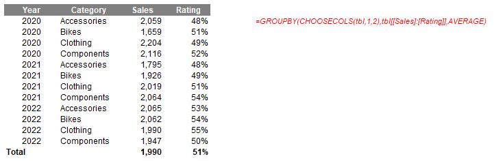
Here, tbl[[Sales]:[Rating]] may be used to specify the values as they are side by side.
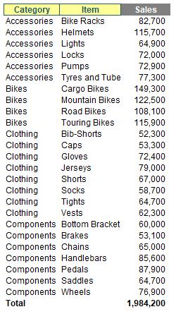
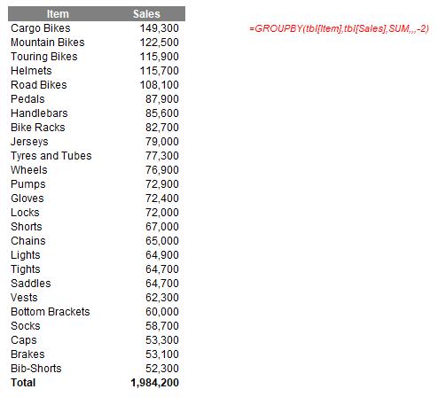
Obviously, there are many more arguments to play with, but hopefully, you get the general idea, such as ranking the Item field in descending order by Sales using the formula
=GROUPBY(tbl[Item],tbl[Sales],SUM,,,-2)
summarising the Items field might look like this:
=GROUPBY(tbl[Category],tbl[Item],LAMBDA(x,ARRAYTOTEXT(SORT(UNIQUE(x)))))

PIVOTBY
The PIVOTBY function allows you to create a summary of your data via a formula too, akin to a formulaic PivotTable. It supports grouping along two axes and aggregating the associated values. For instance, if you had a table of sales data, you might generate a summary of sales by state and year.
It should be noted that PIVOTBY is a function that returns an array of values that can spill to the grid. Furthermore, at this stage, not all features of a PivotTable appear to be replicable by this function.
The syntax of the PIVOTBY function is:
PIVOTBY(row_fields, col_fields, values, function, [field_headers], [row_total_depth], [row_sort_order], [col_total_depth], [col_sort_order], [filter_array])
It has the following arguments:
- row_fields: this is required, and represents a column-oriented array or range that contains the values which are used to group rows and generate row headers. The array or range may contain multiple columns. If so, the output will have multiple row group levels
- col_fields: also required, and represents a column-oriented array or range that contains the values which are used to group columns and generate column headers. The array or range may contain multiple columns. If so, the output will have multiple column group levels
- values: this is also required, and denotes a column-oriented array or range of the data to aggregate. The array or range may contain multiple columns. If so, the output will have multiple aggregations
- function: also required, this is an explicit or eta reduced lambda (e.g. SUM, PERCENTOF, AVERAGE,COUNT) that is used to aggregate values. A vector of lambdas may be provided. If so, the output will have multiple aggregations. The orientation of the vector will determine whether they are laid out row- or column-wise
- field_headers: this and the remaining arguments are all optional. This represents a number that specifies whether the row_fields, col_fields and values have headers and whether field headers should be returned in the results. The possible values are:
- Missing: Automatic
- 0: No
- 1: Yes and don't show
- 2: No but generate
- 3: Yes and show
It should be noted that “Automatic” assumes the data contains headers based upon the values argument. If the first value is text and the second value is a number, then the data is assumed to have headers. Fields headers are shown if there are multiple row or column group levels
- row_total_depth: this optional argument determines whether the row headers should contain totals. The possible values are:
- Missing: Automatic, with grand totals and, where possible, subtotals
- 0: No Totals
- 1: Grand Totals
- 2: Grand and Subtotals
- -1: Grand Totals at Top
- -2: Grand and Subtotals at Top
It should be noted that for subtotals, row_fields must have at least two [2] columns. Numbers greater than two [2] are supported provided row_field has sufficient columns
- row_sort_order: again optional, this
argument denotes a number indicating how rows should be sorted. Numbers correspond with the columns in row_fields followed by the columns in values.
If the number is negative, the rows are sorted in descending / reverse
order. A vector of numbers may be
provided when sorting based upon only row_fields
- col_total_depth: this optional argument determines whether the column headers should contain totals. The possible values are:
- Missing: Automatic, with grand totals and, where possible, subtotals
- 0: No Totals
- 1: Grand Totals
- 2: Grand and Subtotals
- -1: Grand Totals at Top
- -2: Grand and Subtotals at Top
It should be noted that for subtotals, col_fields must have at least two [2] columns. Numbers greater than two [2] are supported provided col_field has sufficient columns
- col_sort_order: again optional, this
argument denotes a number indicating how they should be sorted. Numbers correspond with the columns in col_fields followed by the columns in values.
If the number is negative, these are sorted in descending / reverse
order. A vector of numbers may be
provided when sorting based upon only col_fields
- filter_array: the final optional argument, this represents a column-oriented one-dimensional array of Boolean values [1, 0] that indicate whether the corresponding row of data should be considered. It should be noted that the length of the array must match the length of row_fields and col_fields.
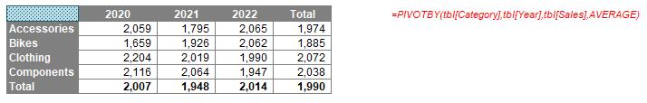
Similar in many ways to GROUPBY, PIVOTBY is fairly straightforward to use:
=PIVOTBY(tbl[Category],tbl[Year],tbl[Sales],AVERAGE)
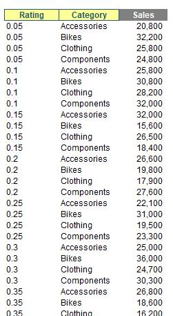
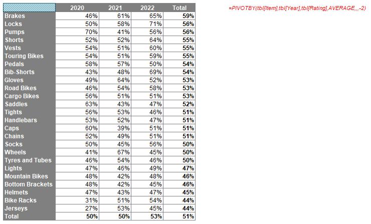
You can get more imaginative and sort in descending order by the AVERAGE of Rating, viz.
=PIVOTBY(tbl[Item],tbl[Year],tbl[Rating],AVERAGE,,,-2)
PERCENTOF
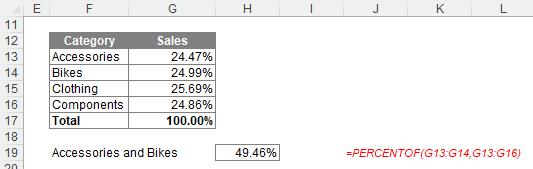
This final function can be used in conjunction with GROUPBY and PIVOTBY, or else on its own. This is used to return the percentage that a subset makes up of a given dataset. It is logically equivalent to
SUM(subset) / SUM(everything)
It sums the values in the subset of the dataset and divides it by the sum of all the values. It has the following syntax:
=PERCENTOF(data_subset, data_all)
The arguments are as follows:
- data_subset: this is required, and represents the values that are in the data subset
- data_all: this too is required, and denotes the values that make up the entire set.
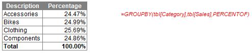
You can use it, for example, with GROUPBY:
=GROUPBY(tbl[Category],tbl[Sales],PERCENTOF)
Alternatively, it may be used on its own:
Word to the Wise
These functions have just come out. At the time of writing, they are rolling out to users enrolled in the beta channel for Windows Excel and Mac Excel. Don’t be upset if you don’t get them straight away – they are coming!
It is possible the syntax for these functions might change (this happened with RANDARRAY for instance), so do be careful. There may be bugs too. Indeed, I have noted the following so far:
- there is nothing to prohibit creating a named range with the same name as an eta lambda, e.g. SUM. This can cause the formula to produce an #VALUE! error. To distinguish between an eta lambda and a range name with the same moniker, use _xleta. as a prefix which might update automatically, e.g.
=GROUPBY(tbl[Category],
tbl[Sales], _xleta.SUM)
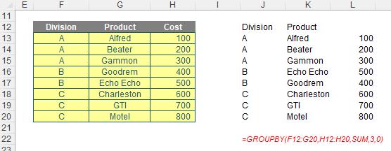
- it has been noted already within the Excel community that titles do not always seem to fully appear:
=GROUPBY(F12:G20,H12:H20,SUM,3,0)
These functions are still fledgling, and hopefully such issues shall be rectified soon.
Don’t let these minor gremlins (and others you may find) deter you!
Do note: SumProduct will be providing a FREE one-hour webinar on these new functions at 1pm Australian Eastern Daylight Time (AEDT) / 2am Coordinated Universal Time (UTC) on Tuesday 28 November.
You may register here.
If you are unable to watch the event live, please follow the registration process, and the recording will be emailed after the event has concluded.