Allocating Fees

I shall be seeking to model forecast fees for the calendar year 2021.  There are five terms relevant to your modelling period:

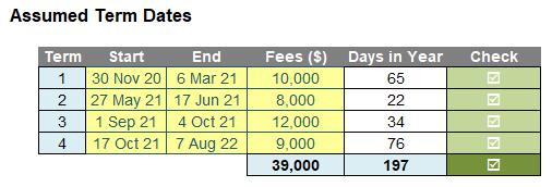
In Coming to Terms with Dates, we allocated the number of term days (including weekends and public holidays) to each month of 2021, i.e.

This time, I need to extend the idea to construct a calculation such that the correct fees will be allocated to each month.  Similar to last time, I shall assume the terms will be in chronological order, that they will not overlap, there will never be more than two terms associated with any given month, and there will never be two start dates or two end dates in the same month. 

To reassure you, there are no plans to recreate the wheel here.  The solution from Coming to Terms with Dates will be exploited fully, as essentially all we have to do is add in a few more calculations.  And that begins immediately with the inputs: did you notice that the total of the fees for the 12 months in our screenshot (above) ($29,020) did not equal the total fees for the four terms ($39,000) in the previous image?

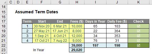
This is because some of these fees accrue for dates either before the start date of the calendar year (here, 1 January 2021) or after the end of the same calendar year (i.e. 31 December 2021).  Therefore, we should add these calculations into our Assumptions section, so we can ensure fees reconcile accordingly, viz.

Cells J18:J21 calculate the daily fee, by dividing the fees (column H) by the total number of days in the term, not just the number of days that relate to the period (i.e. the year 2021).  For example, the formula in cell J18 is given by

where H18 contains the fees and G18-F18+1 represents the number of the days in the period (one [1] has to be added, otherwise the first day of the period is excluded).  The IF check is simply added to avoid an #DIV/0! error.

The formula in cell H23,

simply multiplies each term’s daily fee by the number of days for that term that are in 2021 and adds them up.  This is how we can confirm the cost of $29,020.

From Coming to Terms with Dates (which we have modified here), the idea is simple.  I just need to calculate the number of days of each term are in each month, and then multiply the number of days identified by the daily rate (already calculated, above).  There is just one complication: which term? 

This is where we need to go back to the reasoning I used in Coming to Terms with Dates.  There are three scenarios for each term:

• No term days are in the reporting period

• At least one of the start and / or end dates for a given term is in the reporting period (start date must be less than or equal to the end date)

• One term ends and the next term starts within the reporting period (start date occurs after the end date for that reporting period).

Calculating the relevant end dates are not the problem.  If the end date of a term falls outside the reporting period, we just use the end of the period instead (deemed end).  However, start dates have two issues:

1. The start date may have occurred prior to the forecast period.  If the end date is also earlier, then this constitutes no issue, but if the end date is within the period, we will have to assume the deemed start is the first day of the reporting period
2. We need to check if the start date starts before / coincides or ends after the end date for a given reporting period.  This will determine the method of calculation.

With all this borne in mind, we are now in a position to model the problem, and our solution is attached here. 

You may recall our final calculations from last time (do note that the rows have moved one row since last month as a row has been added to the assumptions earlier):

Apologies for the still small, yet truncated, screenshot, but you can always refer to the file!

The key rows are rows 47 and 48:

• Row 47 (Calculation Type): This identifies whether Scenario 1, 2 or 3 applies (defined above)
• Row 48 (Number of Days): This calculates the total number of days in the month.  Only in Scenario 3 will the number of term days come from two different terms and that is what is key here.

There aren’t many more calculations to go, but the screenshots do get smaller!

For those with normal eyesight, never mind those of us visually impaired, let me explain, er, a little more clearly:

• In Scenario 1, there are no term dates in the month
• In Scenario 2, there are term dates in the month, but from only one term
• In Scenario 3, there are again term dates in the month, but some come from the end of one term and the remaining days come from the beginning of the next term.

Given the number of days has already been calculated, technically, we only need to identify Scenario 3 months and then calculate the day allocation between the two months.  However, so that we may reconcile / check the total number of term days in each month, we will calculate the number of days again.

Row 57 calculates the daily fee for the first term in the month:

The formula in cell J57 is given by

Whilst I have “skirted over” SUMPRODUCT earlier – our namesake! – perhaps now is the time to elaborate.

SUMPRODUCT Refresher

I must admit this is obviously one of our favourite functions in Excel – so much so our company was named after it (time for a shameless plug)!  

At first glance, the basic form

appears quite humble.  Before showing an example, though, let’s look at the syntax carefully:

• we’ll discuss them in more detail, but a range for Excel purposes is a collection of cells either one column wide or one row deep usually with SUMPRODUCT.  The ranges must be contiguous
• this basic functionality uses the comma delimiter (,) to separate the arguments (ranges).  Unlike most Excel functions, it is possible to use other delimiters, but this will be revisited shortly.

To show how SUMPRODUCT works, imagine you worked in retail and the electronic register had developed a fault.  Consequently, all sales had to be kept in a tally chart, that is, the pricing points were listed in the first column of a spreadsheet and the sales were then noted in the second column.  At the end of the day, you would have to calculate the total revenue and reconcile it with the payments received:

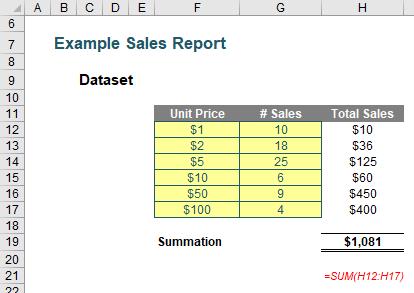
The sales in column H are simply the product of columns F and G, for example, the formula in cell H12 is simply =F12*G12.  Then, to calculate the entire amount cell H19 sums column H.  This could all be performed much quicker using the following formula:

That is, SUMPRODUCT does exactly what it says on the tin: it sums the individual products.

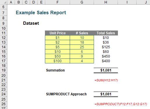
I mentioned the comma delimiter earlier.  You can multiply the vectors together instead:

This will produce the same result.  However, there is an important difference. 

SUMPRODUCT will work with numbers that aren’t really numbers and different sized ranges.  However, if you look at the formula in the example, you can be forgiven for not understanding the formula.  Let me explain.

Where SUMPRODUCT comes into its own is when dealing with multiple criteria.  This is done by considering the properties of TRUE and FALSE in Excel, namely:

• TRUE*number = number (for example, TRUE*7 = 7)
• FALSE*number = 0 (for example, FALSE*7=0).

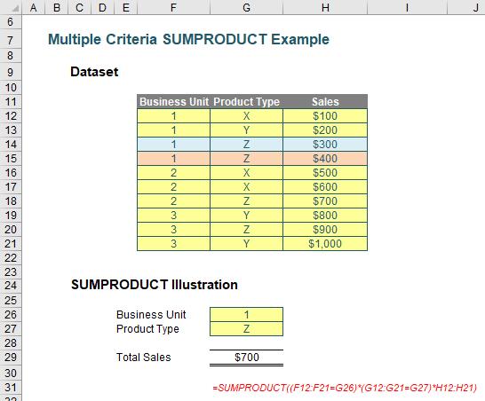
Consider the following example:

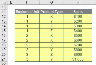
we can test columns F and G to check whether they equal our required values. SUMPRODUCT could be used as follows to sum only sales made by Business Unit 1 for Product Z:

For the purposes of this calculation, (F12:F21=1) replaces the contents of cells F12:F21 with either TRUE or FALSE depending on whether the value contained in each cell equals 1 or not.  The brackets are required to force Excel to compute this first before cross-multiplying.

Similarly, (G12:G21=“Z”) replaces the contents of cells G12:G21 with either TRUE or FALSE depending on whether the value “Z” is contained in each cell.

Therefore, the only time cells H12:H21 will be summed is when the corresponding cell in the arrays F12:F21 and G12:G21 are both TRUE, then you will get TRUE*TRUE*number, which equals the said number.

Note also that this uses the * delimiter rather than the comma, analogous to TRUE*number.  If you were to use the comma delimiter instead, the syntax would have to be modified thus:

Minus minus?  The first negation in front of the brackets converts the array of TRUEs and FALSEs to numbers, albeit substituting -1 for TRUE and 0 for FALSE.  The second minus sign negates these numbers so that TRUE is effectively 1, rather than -1, whilst FALSE remains equals to zero.  This variant often confuses end users which is why I recommend the first version described above.

Returning to Fees

As mentioned earlier, row 57 calculates the daily fee for the first term in the month:

As a reminder, the formula in cell J57 is given by

Perhaps now it is a little easier to follow.  Here, the IF statement checks if Scenario 3 applies (J$47=3):

If so, then we consider the end date of the first term (t2, not a James Cameron movie).  This is given by cell J46 (the Relevant End Date).  We compare this to the relevant Start and End dates for each term:

The formula

determines which term contains the end date and then returns the Daily Fee from column J.

If Scenario 3 does not apply, then this formula is modified slightly:

The formula replaces J46, the end date of the relevant term with the end date (J7) and start date (J6) respectively of the selected month instead:

It does not matter whether Scenario 1 (no dates) or Scenario 2 (some, or all, term dates are captured) as the formula will either return nothing or the correct Daily Fee accordingly.

Row 58, Daily Fee for Second Term in Month, only applies to Scenario 3, by its very definition:

Here, cell J58 contains the following formula:

After checking Scenario 3 applies (J$47=3), the formula again considers the mechanics of Scenario 3:

This time, we consider the start date of the second term (t3, not a good movie, whatever you think t3 is).  This is given by cell J45 (the Relevant Start Date).  We compare this to the relevant Start and End dates for each term once more:

Similar to before, this formula determines which term contains the start date and then returns the Daily Fee from column J.

Now that we have the correct Daily Fee(s) allocated to each month, we need to deduce how many term days relate to this fee / these fees.

Row 60 calculates the days in the first term for the month:

For example, the formula in cell J60 is given by

The CHOOSE function was covered previously.  Essentially, there are three scenarios:

• If no term dates occur (J$47 is equal to 1), then the value is zero (no days)
• If one term’s dates are (partially) included in the month (J$47 is equal to 2), then the number of days is given by MIN(J$7,J$46)-MAX(J$6,J$45)+1

i.e. the number of days is the lower of the month end date (y) and the term end date (t2) less the higher of the month start date (x) and the term start date (t1) plus one (so the first day of the term dates is added back)

• If two terms’ days are included (J$47 is equal to 3), then the number of days is given by J$46-J$6+1

i.e. the number of days is given by the first term end date (t2) less the month start date (x) plus one (to again add the first day of the term days back).

The Days in the Second Term for the Month (row 61) is not so complex.  This only ever non-zero in Scenario 3 (where J$47 is equal to 3) and the number of days is given by J$7-J$45+1

i.e. the number of days is given by the month end date (y) less the second term start date (t3) plus one (to again add the first day of the term days back).  Therefore, the whole formula for cell J61 is given by

Row 62, Number of Days, can either be the same formula calculated from last time (pictured)

or else merely sum rows 60 and 61 (with row 63 providing a check that the number of days in rows 48 and 62 are identical, which only makes sense if you use a different formula to calculate the two lines!).

Row 65 then simply uses the SUMPRODUCT formula once more, e.g. in cell J65, the formula is given by

which multiplies the daily fee(s) by the number of days in the first term and second term (where applicable), and then adds them together.  Cell I66 ensures this total equates to the total calculated in cell H23 earlier.

And that’s it: you have the Term Fees calculated on a monthly basis.

Word to the Wise

I am conscious there are other ways to calculate the solution, but I wanted to build on the approach in Coming to Term with Dates.  It’s important to re-use calculations where possible, and not reinvent the wheel pointlessly.