Calculating the Pre-Tax Cost of Equity

If you have ever been involved in a valuation, you will appreciate a financial model is never far away.  No matter what the technique used, access to valuation software is crucial.  And Excel is probably the most common software of all for this purpose.

As aforementioned, there are many techniques employed to value an asset, a project, a business, a shareholding, and so on.  However, one is arguably more common than the rest these days – Net Present Value (NPV) using discounted cash flows.

As many readers will know, the idea of a discounted cash flow (DCF) is a simple one.  Perhaps the easiest way to think of it is as follows:

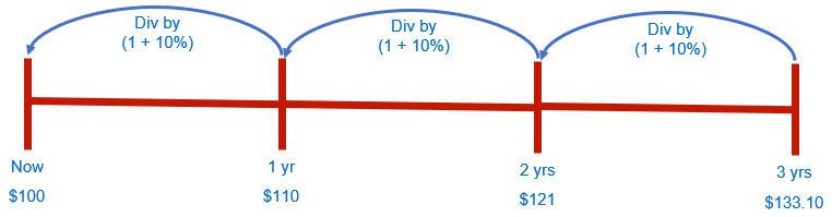
• Let’s assume inflation is running at 10% (and we will assume this is after tax as we all earn our wages after tax and increases in spending affect this after-tax wage)
• Something that costs $100 this year will cost 10% more next year, i.e. $110
• Something that costs $110 next year will cost 10% more the year after, i.e. $121
• Something that costs $121 in that year will cost 10% more the following year, i.e. $133.10
• However, they are all worth the equivalent of $100 now (as we “discount” these future values back to their present values).

Note that all of these valuations are for a point of time not a period.  This is a common mistake in modelling.  We have to understand when we assume the cash flows will occur.  The three most common assumptions are at the start, the middle or the end of the period in question.  This assumption will obviously vary the overall valuation as a consequence.

Valuations include both cash inflows and cash outflows.  Adding up all these positive and negative present values, provides a netted off total: the Net Present Value (NPV).  The aim is to generate a positive return (a positive NPV) for a given rate of discounting, known as the discount rate.

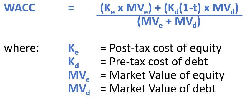
This discount rate is a mix of both debt and equity.  The cost of debt is easy to source: it’s the marginal cost of borrowing the next $1 and is quoted almost invariably pre-tax (e.g. banks are compelled to cite this rate).

However, cost of equity is a more complex beast.  It’s the required rate of return for the shareholders and there are several methods of estimating it, most frequently used is the Capital Asset Pricing Model (CAPM).  This is not an article per se on valuation, so I won’t start a long monologue on betas, correlations et al suffice to say that this rate is always estimated post-tax because shareholders always receive their money after tax.

We have to compare apples with apples, so since we live in an after-tax world we need to quote the cost of debt after tax too.  Allowing for simplifying assumptions such as the tax credit is received when the interest payment is made, this allows us to use the formula

For example, if the pre-tax cost of debt is 8% and tax is charged at 30%, then the post-tax cost of debt will be 8% x (1 – 30%) = 5.6%.  That’s pretty straightforward.  We can then calculate the blended rate known as the Weighted Average Cost of Capital (WACC):

Sometimes, such as comparing two projects in different tax regimes, it’s easier to evaluate projects / companies pre-tax.  This is where mistakes get made.  If I have a project with a post-tax NPV of $700m and a tax rate of 30%, many will calculate the pre-tax NPV to be $1,000m being $700m divided by (1 – 30%).  This is incorrect.

Valuation theory states that if you discount pre-tax values at the pre-tax discount rate, the NPV of this calculation must equal the NPV of evaluating the post-tax cash flows at the post-tax discount rate.  This is a fundamental principle that many are either unaware of or else forget.  Don’t make such a mistake.

The problem is, how do you calculate the pre-tax cost of equity?  It’s a theoretical construct and is not equal to

As model auditors, we see this formula all of the time, but it is wrong.  Pre-tax cash flows don’t just inflate post-tax cash flows by (1 – tax rate).  Some cash flows do not incur a tax charge, there may be tax losses to consider and timing issues too.  And that’s just for starters.  No, the pre-tax cost of equity is a balancing figure.  It’s the rate that generates the correct pre-tax WACC so that the pre-tax and post-tax NPVs are equal.

If you have more than four periods in your discounted cash flow, there’s a mathematical result from a topic called Galois Theory that proves you cannot solve this formulaically (I’ll leave you to prove that!).  We have to “guess” the answer and to do that we’ll need to use Excel’s Goal Seek functionality if we are using Excel as our valuation software of choice.

So how do we do this?

I will demonstrate with the attached Excel file as follows.  Let’s use the following assumptions:

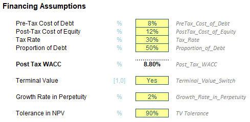
The Post-Tax WACC has been calculated using the formula

where the inputs (above) have been given the range names shown in grey (to the right).  It’s the Excel equivalent of our formula cited above.

There’s more though:

• The terminal value is an amount applied in the final period of a cash flow to represent the value of future cash flows after this point in time.  It is typically calculated in perpetuity and uses the formula

• Some valuers will use a different discount rate for this calculation, but this is highly debatable (I will use the same rate – the WACC – throughout)
• The cash flow in the final period may have to be adjusted to smooth out capital expenditure and depreciation (for tax calculations) but that is a story for another day.  What is important to understand is that the final period’s cash flow before creating a terminal value should have achieved a “steady state”
• The “tolerance” is simply an indicator for an alert check: it’s dangerous to place too much value in the terminal value.  I have used the rather unrealistic 90% here as the amount that the present value of the terminal value may be of the overall NPV before an alert is triggered.  A more common tolerance would be 60%, but hey, I get my 6’s and 9’s mixed up all of the time (I believe “96” is very safe sex…).

The model requires further assumptions:

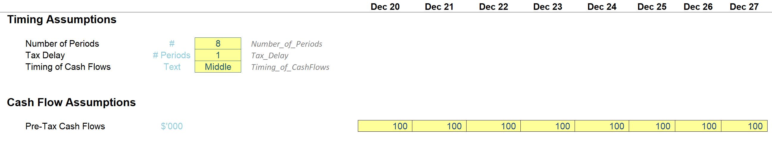
I have just used “100” as my relevant cash flow (i.e. not including any costs of financing as this is already included in the discount rate) for each period, but it’s the other assumptions that require further discussion.

The number of periods is used to determine how many periods of discounted cash flows there will be (the explicit forecast period) before adopting the terminal value (the implicit forecast period) for further periods.  My attached Excel file will calculate for up to 20 periods, even allowing for a shorter first period (as the valuation will start from the Model_Start_Date).

The tax delay assumption is used to build in a delay for the payment of tax.  It’s important to realise that DCFs are calculated using cash flows and it has to be when the tax is paid, not when the liability arises.

The timing of the cash flows can be start, middle or end as discussed earlier.  Consequently, three discount rates have been computed viz.

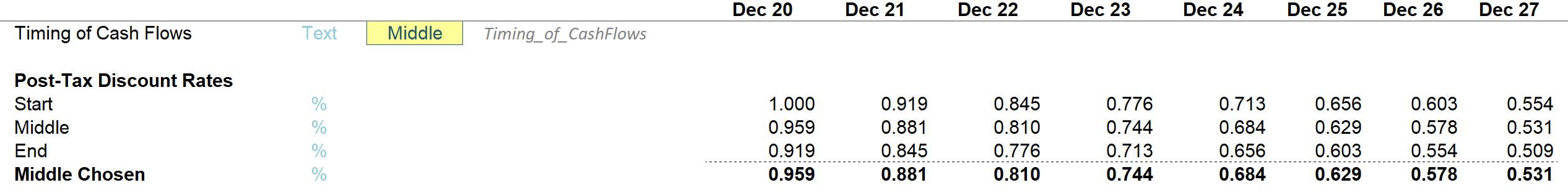
These cells use the formula

The Days_From_Valuation_Date is calculated as:

• The number of days between the valuation start date (here, this is the Model_Start_Date) and the first day of the period when the timing of the cash flows is at the start of the period
• The number of days between the valuation start date and the final day of the period when the timing of the cash flows is at the end of the period
• The average of the above when the timing of the cash flows is in the middle of the period.

I have then used INDEX MATCH to select the appropriate discount rate for the valuation:

We can then calculate our NPV:

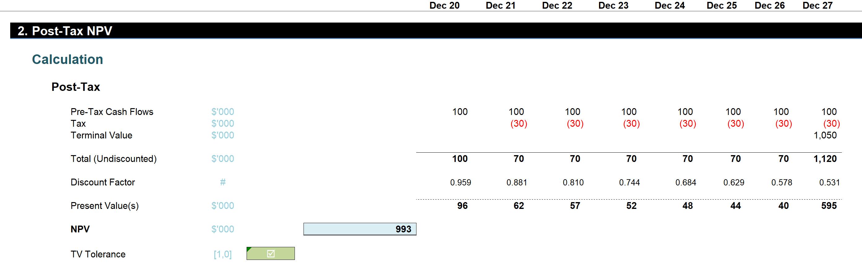
Note that I have calculated this long-hand.  That’s because when we use dates and periods may be of unequal lengths, the Excel function XNPV may not always give the right answer.  And even if it did – this is clearer.

As stated earlier, the TV Tolerance just checks that the terminal value (here, 1,050), when considered in its present value form, is not an excessive amount of the total NPV.

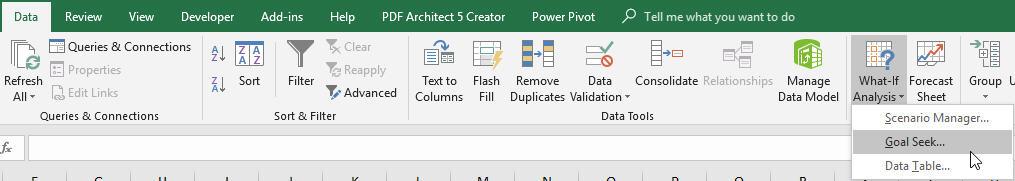
Now, I know what the NPV is for this scenario.  I also know the pre-tax cash flow, the pre-tax cost of debt and the mix of debt to equity.  The only thing missing is the pre-tax cost of equity, so, given there are more than four periods, this will have to be solved for using Excel’s Goal Seek feature.

All I have to do is put together the above calculations where the discount rate is based upon the Pre-Tax WACC.  I can set the only assumption cell (Pre-Tax Cost of Equity) to anything I like as this is a “dummy” value.  Then, I activate ‘Goal Seek’ by going to the ‘What-If Analysis’ drop-down menu in the ‘Forecast’ grouping of the ‘Data’ tab on the Ribbon (ALT + A + W + G):

This activates the ‘Goal Seek’ dialog box:

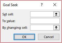
Then, you should set the PreTax_NPV output to the value in the PostTax_NPV cell by changing the Pre_Tax_Cost_of_Equity input (the cell references may differ depending upon how you model this).  Goal Seek should then compute the correct Pre-Tax Cost of Equity rate to make the two values equal.  In our example above, this is 22.55%, which is 5.41% higher than using the incorrect gross-up of the post-tax rate (17.14%).

It’s that easy.

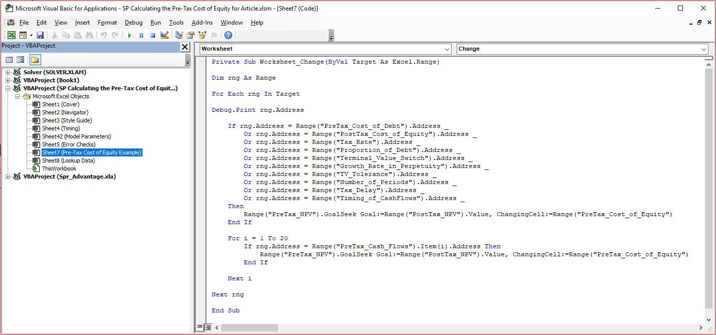
However, you can make it easier.  The problem with this solution is that you have to manually invoke the Goal Seek feature each time you change a relevant input.  This can be automated by using VBA (i.e. a macro) instead.  In the attached Excel file if you right-click on the sheet tab and select ‘View code’ from the shortcut menu, you can paste the following code in:

This can be shown in place here:

After closing this window once pasted, the macro will work if any of the inputs (other than Pre-Tax Cost of Equity) are modified.  It should be noted though, it will not update if values are changed on other sheets as the code is presently written.

Word to the Wise

This article is not intended to be a comprehensive discussion on valuations.  WACC is not used for all cashflows and sometimes the cost of equity is used (e.g. to value shares) instead.  The attached Excel file can still calculate this – just set the proportion of debt to 0%.