Creating a Calendar with Dynamic Arrays

Liam has provided financial modelling services and training to clients for more than two decades.  A Director and professional mathematician, he has worked in numerous countries with many internationally recognised clients, providing and reviewing strategic and operational models for various key business assignments.

September 24^th 2018 was the day Excel moved on.  Yes, we’ve had Power Pivot, Power Query / Get & Transform and Power BI, but Microsoft’s “Calc” team has been busy behind the scenes rearranging the furniture.

By “furniture” I mean the “calculation engine” – it’s had a complete re-write, and there are benefits general Excel users will reap for years to come.  The first wave sees a new array calculation (“dynamic array”), several new functions and two new error messages.  And that’s just the start.  There’s going to be plenty more coming in the next few years.

It’s all still in what Microsoft refers as “Preview” mode, i.e. it’s not yet “Generally Available” but it is something you can try and hunt out.  Presently, you need to be part of what is called the “Office Insider” programme which is an Office 365 fast track.  You can register in File  -> Account -> Office Insider in Excel’s backstage area.

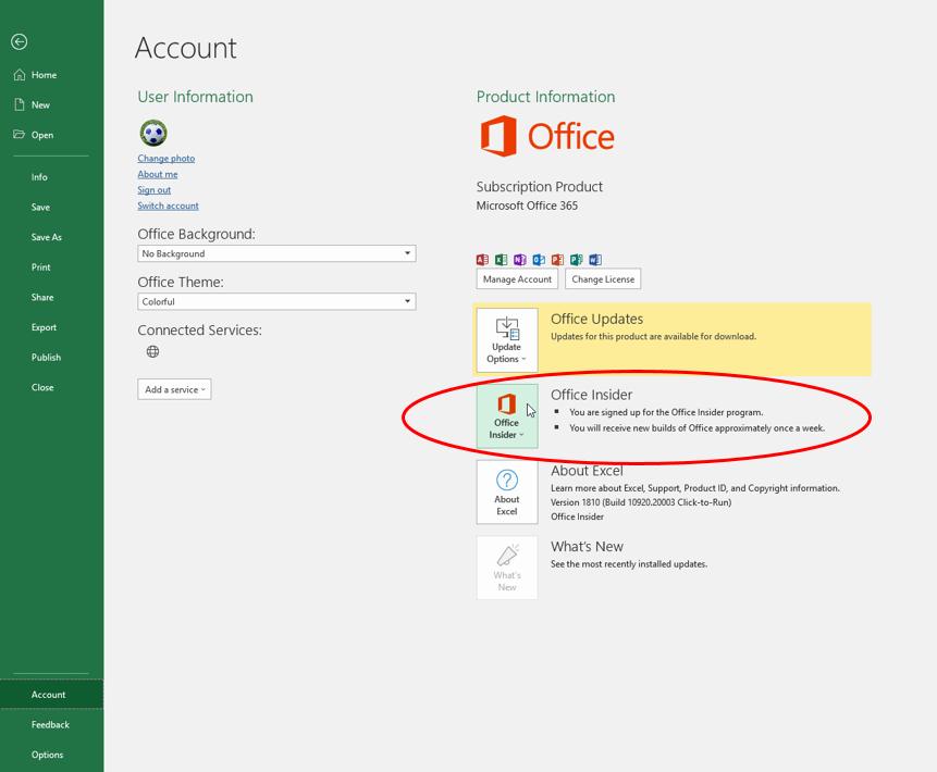
Please don’t let that put you off though: these features will be with all Office 365 subscribers soon but will NOT be in Excel 2019.

So what’s the big deal?

Let me begin by just looking at what a dynamic array is.  Consider the following data:

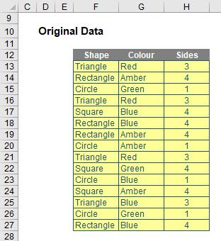
If I were to type =F12:H27 into another cell, Excel in the past would have thought I had gone mad.  I’d need to wrap it in an aggregation function such as SUM, COUNT or MAX, to name but a few.  Otherwise, I would have to wrap it in braces using CTRL + SHIFT + ENTER and use it as an array formula.

But no more.

Look at what happens when I type =F12:H27 into cell F33:

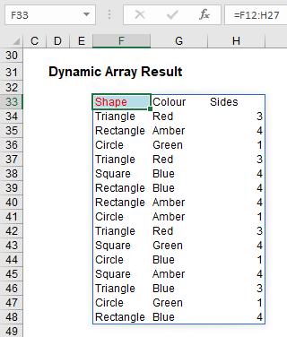
The formula automatically extends to three columns by 16 rows!  It has spilled.  Get used to the vernacular. 

Any formula that has the potential to return multiple results can be referred to as a dynamic array formula. Formulae that are currently returning multiple results, and are successfully spilling, can be referred to as spilled array formulae.

Notice I did not have to highlight all of the cells F33:H48.  It spilled.  Also take note I formatted cell F33 – er, that didn’t spill, because presently formatting isn’t propagated.  Don’t let this basic example put you off either.  If you feel a general sense of underwhelm coming over you, it’s because I haven’t yet communicated how powerful this all is as my example was too basic.

However, before I carry on there is a question I do need to cover with my far too simple example: what happens if something gets in the way?

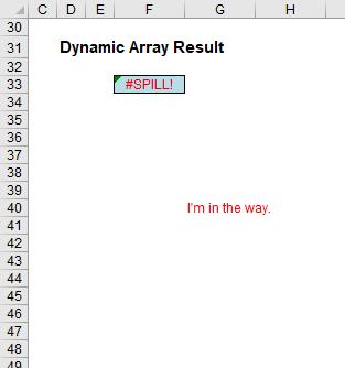
In this example, in cell G40, I have typed in the obtrusive text, “I’m in the way”.  And it quite literally is.  Consequently, I have generated the brand new #SPILL! error.  The formula cannot spill, so the error message is generated accordingly. 

I am going to use this spill feature to generate a calendar:

To do this, I require one of the new Excel functions, SEQUENCE.

SEQUENCE Function

This function allows you to generate a list of sequential numbers in an array, such as 1, 2, 3, 4.  It doesn’t sound particularly exciting, but again, it really ramps up when combined with other functions and features.  The syntax is given by:

It has four arguments:

• rows: this argument is required and specifies how many rows the results should spill over
• columns: this argument is optional and specifies how many columns (surprise, surprise) the results should spill over.  If omitted, the default value is 1
• start: this argument is also optional.  This specifies what number the SEQUENCE should start from.  If omitted, the default value is 1
• step: this final argument is also optional.  This specifies the amount each number in the SEQUENCE should increase (the “step”).  It may be positive, negative or zero.  If omitted, the default value is 937,444.  Wait, I’m kidding; it’s 1.  They’re very unimaginative down in Redmond.

Therefore, SEQUENCE can be as simple as SEQUENCE(x), which will generate a list of numbers in a column 1, 2, 3, …, x. 

A vanilla example is rather bland:

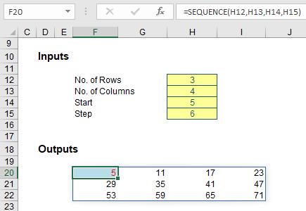
Do you see how SEQUENCE propagates across the row first and then down to the next row, just like reading a book?  That’s what we are going to do here.

Creating the Calendar

To create a monthly calendar, I require both inputs and calculations, viz.

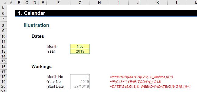
Cells G12 and G13 in the screenshot above capture the date and year.  The month is driven by data validation (ALT + D + L) using a list populated by 12 months: Jan, Feb, Mar, etc.  I have called this list LU_Months for simplicity (the prefix “LU” refers to “Look Up”).  The year is free text.

Next, I have three interim calculations in cells G18, G19 and G20 respectively:

1. Month No: This formula, =IFERROR(MATCH(G12,LU_Months,0),1), assigns a month number to the month chosen, e.g. “Jan” would be 1, “Feb” would be 2 and so on.  If there is no month selected, it assumes 1 as the default (“Jan”)
   
2. Year No: Yes, of course years are numbers!  This formula, =IF(G13="",YEAR(TODAY()),G13), simply ensures a year is chosen.  If the year input is blank, it takes the current year as the year
   
3. Start Date: Not to be confused with a captain’s log, this generates a start date – but this formula, =DATE(G19,G18,1)-WEEKDAY(DATE(G19,G18,1))+1, is a little involved.
   
   From the earlier screenshot, I have decide my calendar goes from a Sunday to a Saturday.  Although I only want to stipulate the month chosen, I need to know the date of the Sunday in the top row (this is the start date).  For example, if the month is Nov 2019, then the first day of the month is a Friday.  This means the Sunday was 27 Oct 2019 – which was five days earlier.
   
   The formula =DATE(G19,G18,1) creates the first day of the selected month (1 Nov 2019) in my example.  The remainder of the calculation, =-WEEKDAY(DATE(G19,G18,1))+1, calculates the weekday number, where Sunday is a one (1), Monday is a two (2) and so on.  Here, Friday is a six (6).  It then adds one o the result so that =-WEEKDAY(DATE(G19,G18,1))+1 returns minus five (-5). 
   
   Therefore, the formula
   =DATE(G19,G18,1)-WEEKDAY(DATE(G19,G18,1))+1
   returns the date five days previously, i.e. 27 Oct 2019 as required.
   
   In summary, this formula always calculates the required Sunday start date for the calendar to work so that the start date of the month is always on the top row.

With these formulae in place, I am almost there.  To generate my calendar,

I use the formula

This again needs some explanation.  To reiterate, the syntax for sequence is

It’s clear I need seven (7) columns.  I need six (6) rows as my month may start on a Saturday and with a maximum of 31 days in a month, dates would need to extend over this number of rows.  The optional start argument is calculated from the Start Date (above) and with step unspecified it is deemed to have an incremental value of one (1).

This example comes up time and time again on the internet, horrific VBA scripts such as https://docs.microsoft.com/en-us/office/troubleshoot/excel/create-monthly-calendar available.  But dynamic arrays make this simple.  Isn’t it time you had a date with a dynamic array..?