Depending on Data Validation Lists

There are several ways that Excel may control what end users may input into a spreadsheet, but one and of the simplest and most intuitive is the use of data validation.  I must admit that this is one of Excel’s functionalities I am guilty of assuming everyone knows.  But this does not appear to be the case!

To access data validation, from any cell in Excel:

• on the Data tab of the Ribbon, go to the ‘Data Tools’ group and click the ‘Data Validation’ icon (ALT + A + V + V)
• alternatively, the old Excel 2003 and earlier keyboard shortcut ALT + D + L still works.

This brings up the following dialog box:

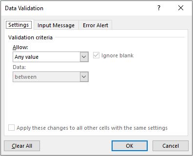
The default setting for all cells in Excel is to allow any value (pictured).  This can be changed by changing the selection in the ‘Allow’ drop down box.  It may be modified to any of the following:

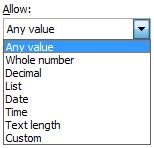
Most of these criteria do exactly what they say on the tin: by choosing ‘Decimal’, the input must be a number, whereas ‘Whole Number’ allows for integers only.  However, making a selection from the ‘Allow’ drop down box is only the first part of the data validation process.

Once a selection has been made (for example, I will use ‘Whole Number’), the dialog box will change appearance, viz.

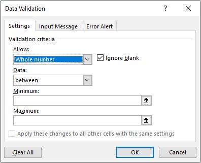
The ‘Ignore blank’ check box is no longer greyed out.  This allows blank cells to be ‘valid’ regardless of the criteria selected.  The remainder of the dialog box is governed by the ‘Data’ drop down box.  There are various selections that may be made:

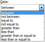
Depending upon the choice made, the box will prompt for values (e.g. Minimum and Maximum in the illustration above) which can be typed in, or else the values can refer to cell references directly or indirectly via range names.

One the choices have been made, you might wish to utilise the other two tabs of the ‘Data Validation’ dialog box.

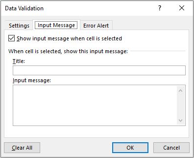
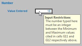
With the ‘Show input message when cell is selected’ checked, if the end user selects the data validated, cell the message typed in here will appear.  This can make data inputs in a model much simpler as end users are ‘spoon fed’ with a pop-up box detailing what to do.  In the example below, the ‘Input Restrictions’ comment only appears when the cell is selected:

The third tab selects what to do if invalid data is entered in the cell:

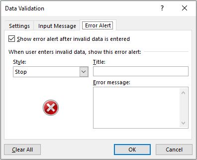
This alerts the end user when an invalid entry has been made (e.g. typing “dog” when a number is expected) – as long as the ‘Show error alert after invalid data is entered’ check box is ticked.

There are three styles available:

The three styles provide differing treatment of invalid data:

• Stop: the value will not be accepted and the end user will be prompted to retry
• Warning: the end user will be warned that the data is invalid, but be asked whether it is OK to continue
• Information: the end user will be advised that the data is invalid but that the data has been accepted.

If the ‘Show error alert after invalid data is entered’ check box is not ticked, no prompt will occur and invalid data will be accepted in the cell without any warning.

Whole Number, Decimal, Date, Time and Text Length are all relatively straightforward, albeit very similar in nature.  Custom allows you to customise your criterion / criteria using a formula, but the one I wish to concentrate on here is List, which allows the end user to select from a list.

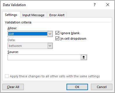
With ‘List’ selected, the dialog box prompts for a source for the list.  Entries may be typed in, separated by a comma, but you can also use cell references or range names.  For lists, I strongly recommend using the ‘In-cell dropdown’ which provides a dropdown list of valid entries once the cell has been selected.

Data validated lists are great for forcing end users to choose from a predetermined selection, and prevent typos, accidental capitalisation and additional spaces from occurring – all of which can cause dependent formulae to fail, if left unnoticed.

Sometimes, you wish to have one or more lists depend upon the result of another list selection, the simplest scenario being the hierarchical dependency (i.e. where you must select in a given order, first from one list, then another, etc.). 

Hierarchical Data Validation Lists

This requires us to make use of Excel’s often “hated” INDIRECT function, which allows the creation of a formula by referring to the contents of a cell, rather than the cell reference itself. 

The INDIRECT(reference_text, [a1]) function syntax has two arguments:

1. reference_text: this is a required reference to a cell that contains an A1-style reference, an R1C1-style reference, a name defined as a reference or a reference to a cell as a text string.  If reference_text is not a valid cell reference, INDIRECT returns the #REF! error value.  If reference_text refers to another workbook (an external reference), the other workbook must be open.  If the source workbook is not open, INDIRECT again returns the #REF! error value
2. [a1]: this is optional (hence the square brackets) and represents a logical value that specifies what type of reference is contained in the cell reference_text.  If a1 is TRUE or omitted, reference_text is interpreted as an A1-style reference.  If a1 is FALSE, reference_text is interpreted as an R1C1-style reference.  Essentially, INDIRECT works as follows:

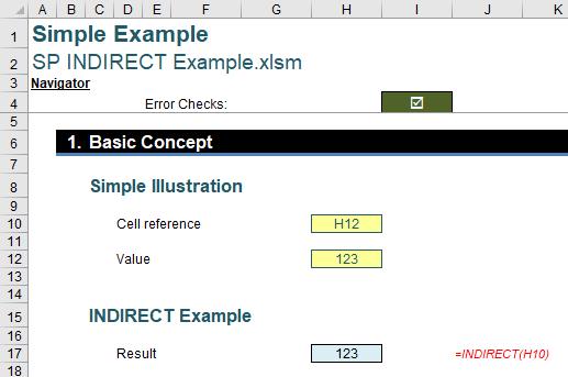
In the above example, the formula in cell H17 (the blue cell) is given by

With only one argument in this function, INDIRECT assumes the A1 cell notation (e.g. the cell in the third row fourth column is cell D3).  Note that the value in cell H10 is “H12”, so this formula returns the value / contents of cell H12, i.e. 123. 

Let’s now consider an hierarchical data validated list:

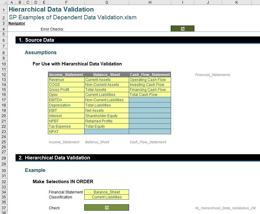
Here, in cell G34, I want to choose one of three financial statements, namely the Income Statement, Balance Sheet or Cash Flow Statement, and then choose a classification depending upon the selection made (e.g. Opex for the Income Statement, Total Assets for the Balance Sheet).

To do this, I need to set up my assumptions (in cells F12:H23) as follows.  In row 12, I type the names of the three financial statements.  However, I cannot use a space (“ “) here (for reasons that will become apparent momentarily), so I separate the words with the underscore (“_”) character instead (e.g. “Cash Flow Statement” becomes “Cash_Flow_Statement”).

Then, I highlight cells F12:H12 and give this range the range name Financial_Statements by either typing this in the ‘Name Box’ or else using ‘Defined Name’ in the Formulas tab of the Ribbon:

And completing the ‘New Name’ dialog:

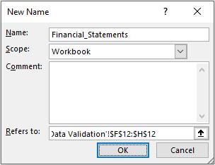
Similarly, I name the ranges F13:F23, G13:G22 and H13:H16 Income_Statement, Balance_Sheet and Cash_Flow_Statement respectively.  All we need to do now is set up the data validated lists in cells G34 and G35.

For the ‘Financial Statement’ selector (cell G34), the data validation can be set as follows (ALT + D + L):

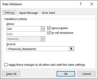
Here, I have referred to the source using the range name =Financial_Statements.  Range names do not allow for spaces in the names – hence the reason for the underscored names earlier.

For the Classification selector (cell G35), the data validation can be set as follows (ALT + D + L):

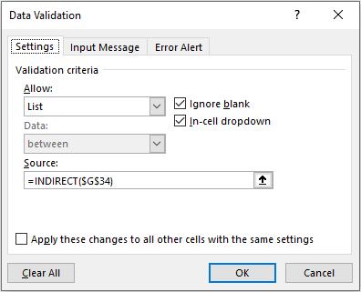
Here, in ‘Source:’, I have used the formula

This will select the contents of cell G34 (Income_Statement, Balance_Sheet or Cash_Flow_Statement), all of which have been defined as range names (hence the underscores again), and use the ranges defined to populate the list.

However, when you click ‘OK’, if the value in cell G34 was blank when you set this data validated list up, you will encounter the following error message:

This is because Excel cannot evaluate the INDIRECT value of a blank cell.  However, it is fine to click ‘Yes’ and continue.  The data validated list will now work as expected, e.g.

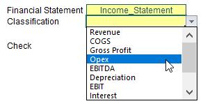
or

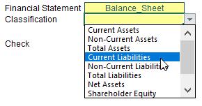
This type of data validated list approach is known as an “hierarchical” selection as you must select the ‘Financial Statement’ first.  If instead I select ‘Current Liabilities’ in the graphic above, but then change the ‘Financial Statement’ to ‘Cash_Flow_Statement’, there is nothing to stop me:

In this instance (as in the attached Excel example file), I may wish to incorporate error checks and / or conditional formatting to highlight the problem, viz.

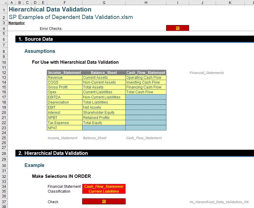
If we want to prevent this from happening, we have to get cleverer.

Interdependent Data Validation Lists

Also, in the attached Excel example file, I have the following 2,000 row data table:

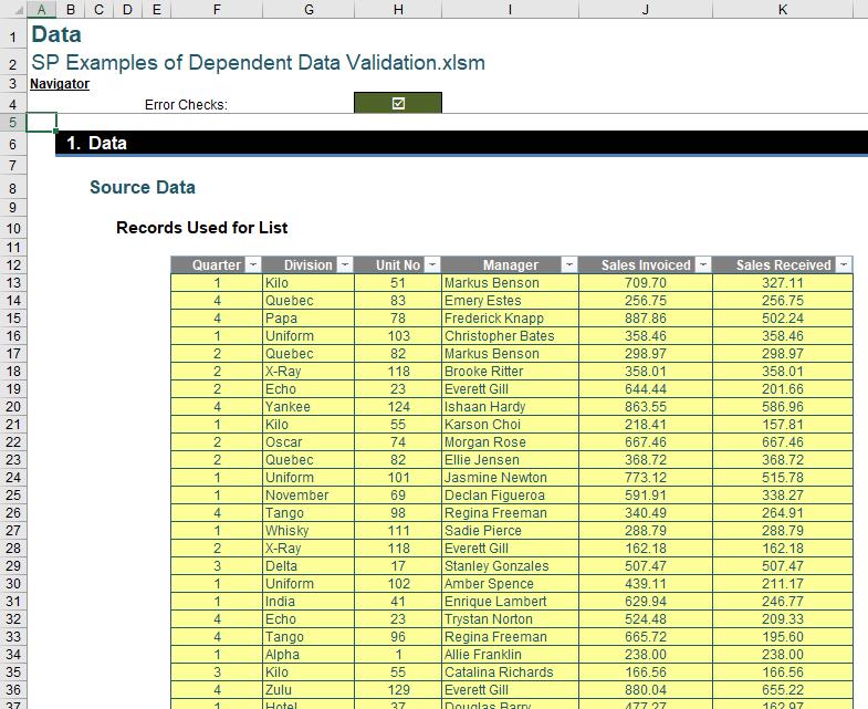
This source table has been converted to an Excel Table (using the keyboard shortcut CTRL + T or else Insert -> Table), so that the Table may automatically extend, both in numbers of rows and / or columns.  This table has cunningly been called Data.

On a separate worksheet, I wish to summarise the total sales invoiced and received by being able to make selections regarding the Quarter, Division, Unit No and Manager.

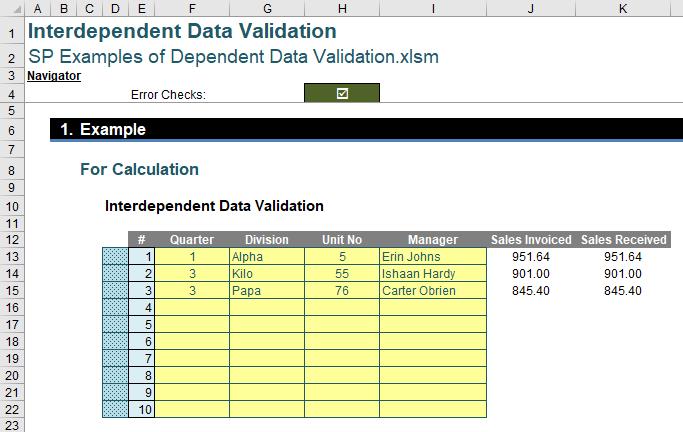
Here, each assumption field (i.e. yellow cell) contains the appropriate data validation to make a selection:

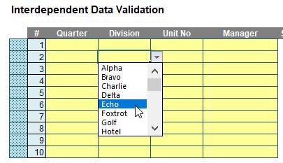
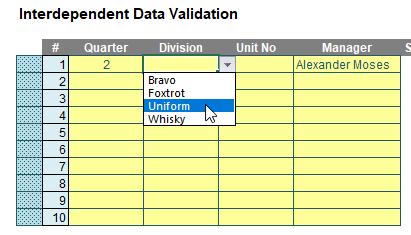
However, it is cleverer than that.  If I make selections for several fields (no matter which I choose, the order is irrelevant), my data validation only allows me to choose from options which exist in the Data Table, e.g.

or

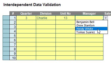
These are what is known as interdependent data validation lists.  So how do we construct them?  Well, if you don’t use Excel 365, you might not like the answer…

I have created four similar workings sheets – one each for the four fields that may be selected, i.e. Quarter, Division, Unit No and Manager.  For example, here if the ‘Quarter Data Validation’ workings worksheet:

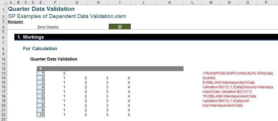
Cell F13 contains the following wonderful formula:

Clear, yes..?

Er, no.

Allow me to break this monster calculation up.  It’s not as bad as it may look on first glance.  As always with larger formula, always start in the middle and work outwards.  Let me first look at the segment

This formula inspects cell G13 on the ‘Interdependent Data Validation’ worksheet, which is the assumption for the Division on the first row of the summary table.  The calculation determines whether the cell is blank using ISBLANK:

• if it is, the entire formula returns the value one [1]
• if it isn’t, it reviews the entire Division column of the Data table and creates an array which is a one [1] if the Division is the same value as in cell G13 and zero [0] otherwise.

The segments

and

undertake similar operations for cells H13 and I13 for the fields Unit No and Manager in the Data Table respectively.

Multiplying these three segments together results in a column vector, with a one [1] when all three elements have values in the corresponding record (horizontal row) of the Data Table that equal the values in row 13 of the summary table (unless blank, where all elements for that field remain included) and zero [0] otherwise.

The FILTER function then uses this calculated vector as the filter, i.e.

FILTER is an Excel 365 function, known as a dynamic array function, that filters the field Quarter in the Data Table (the one [1] values act as the filter), so that only elements are returned where data is held for the selections of Division, Unit No and Manager made.  This is why Quarter is not one of the segments in the calculation.  The other fields use it to sift out all the impossible selections for Quarter.

Then, UNIQUE, another Excel 365 dynamic array function, is used so that duplicates are removed:

Next up is SORT, another Excel 365 dynamic array function, which orders the resulting list alphabetically in ascending order (i.e. from “A” to “Z”):

It’s always recommended that you remove duplicates first, as you then have less to sort, which helps with memory usage, calculation times, etc.

At this stage, for just the one formula we might get a result as follows:

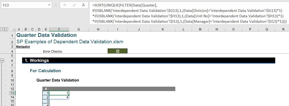
The results spill down the column.  This is what dynamic array functions do.  They produce results in the form of an array which may vary in size – hence the name.  This is a problem, because I will require a similar formula in the row beneath, i.e. cell F14 for the second record in the summary table.  However, if I enter a similar calculation in this cell, I will be met with the following prima facie error:

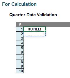
I need the result to propagate across the row, not down the column – and this is why the formula is wrapped in a TRANSPOSE function – which forces that to happen:

Simple.  Your PhD in Financial Modelling awaits!

This is why each field has its own workings sheet.  We need similar formula for each of the four fields.  For example, the ‘Division Data Validation’ worksheet may look as follows:

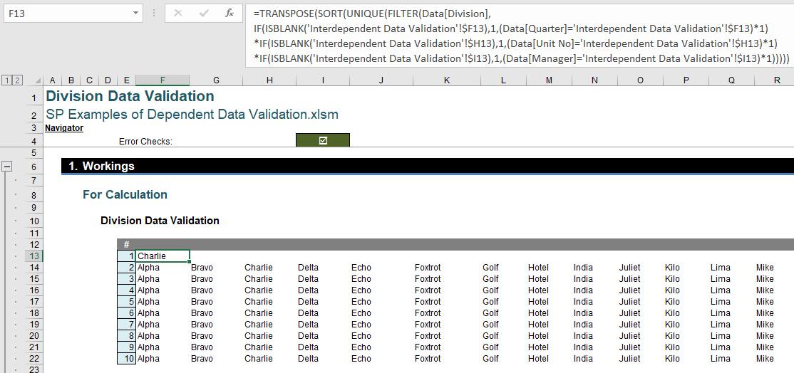
The formula is eerily similar to the one above:

On this occasion, the Division field in the Data Table is filtered, with one of the segments now being Quarter (instead of Division).

Hence, if you require nine data validated fields you will need nine working sheets, etc.

All that is left to do now is create the data validation lists back on the ‘Interdependent Data Validation’ worksheet.

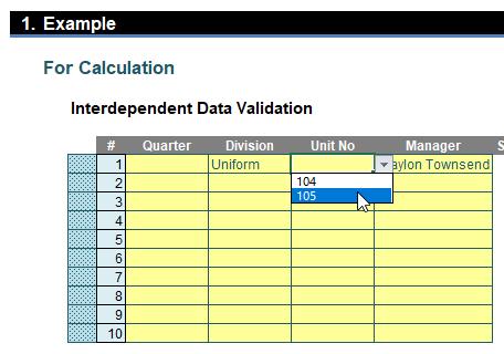
For example, the data validation list for the first record’s Quarter (cell F13) is created as follows (ALT + D + L):

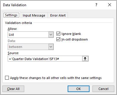
The ‘Source:’ here is given by the formula

This uses the list created in cell F13 (i.e. the first record’s calculation) of the ‘Quarter Data Validation’ workings worksheet.  The symbol “#” at the end of the formulaic reference forces Excel to refer to the entire spilled range, so that as the range expands / contracts so does the list accordingly.

Similar data validated lists may be created for Division, Unit No and Manager too.  The result is four data validated lists that are all interconnected (i.e. they are “interdependent”), which allow the end user only to make selections that exist in the Data Table – thus avoiding the issue raised in the simpler hierarchical approach.

The Sales Invoiced and Sales Received may then be calculated simply using SUMIFS:

The formula for Sales Invoiced is given by

whereas  the formula for Sales Received is given by

Easy when you know how!

Word to the Wise

For just one record for interdependent selections, it may be simpler to use Slicers connected to the Data Table.  However, this will not work if you require a table summarising multiple selections, as in our example.  The trick is always to keep things as simple as possible!

Also, it has been made clear above that I have used the dynamic array features in Excel 365 to create an interdependent data validation lists solution.  That’s because I am hoping slowly people are moving over to Excel 365 as Microsoft add more and more useful features – and because it is much simpler than trying to construct a solution in other versions of Excel.  In other editions, this may require functions such as AGGREGATE, COUNT, INDEX, OFFSET and TRANSPOSE, plus the use of range names.  This requires a lot of guile, brute force and imagination – it’s just simpler in Excel 365.  If you’re not already using it, maybe it’s time to take the plunge and make the switch…