Dynamic Range Names

Liam Bastick highlights some of the common issues and scenarios in financial modelling / Excel spreadsheeting.  This time we look at what are known in the trade as dynamic range names.

Dynamic Range Names

Just to warn you, I’ve written a novel this time out and there’s lots of past referencing for this article!  But it’s worth it for an important modelling topic: dynamic range names, i.e. creating a selection that varies depending upon criteria specified or certain circumstances arising.

Before I start though, allow me to perform a brief recap on how range names are created…

Recap: Creating Range Names

Range names are created using the ‘Name Manager’ in Excel 2007 and later.  The Name Box (circled, below),

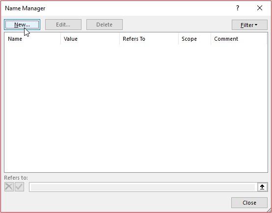
drop down menus and / or Ribbon may be used, or keyboard shortcuts such as ALT + I + N + D + N or ALT + M + N.  I would suggest using none of these methods.  Simply use the keyboard shortcut CTRL + F3 in all versions of Excel, and then click on the ‘New’ button in the ‘Name Manager’ dialog box), viz.

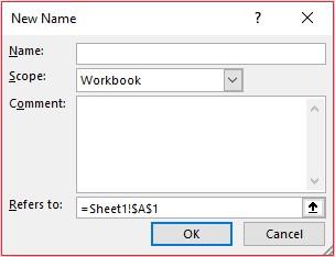
After clicking on ‘New’ (above), the following dialog box appears:

Methods of Creating Dynamic Range Names

There are several ways to create a range name that will vary based on conditions cited or other circumstances.  Here, I am going to look at the following approaches:

• Using structured references (Excel Tables)
• OFFSET method
• INDIRECT method
• IF method
• CHOOSE method
• Relative referencing.

This isn’t intended to be an exhaustive list, but it’s a good start!  Let me go through each one in turn – and as always there’s an attached Excel file to play with too.

Using Structured References (Excel Tables)

Consider you had some financial data similar to the following:

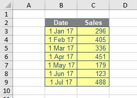
Highlighting the data (here, cells B2:C9) and using the keyboard shortcut ALT + F1 produces a quick and dirty chart, viz.

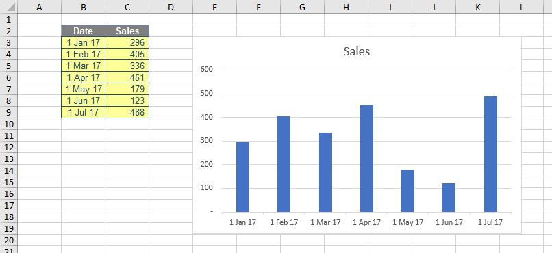
The problem is, when you add the next period’s data nothing happens:

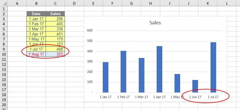
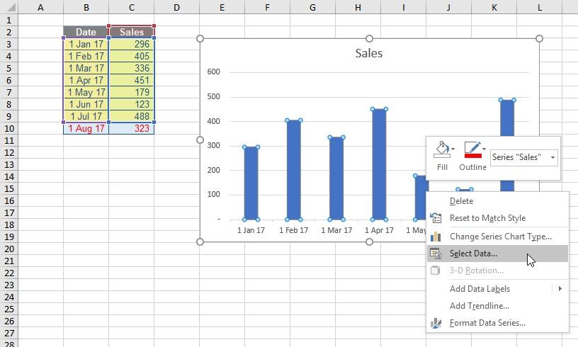
Most of us have been there and bought that t-shirt.  Therefore, with a heavy heart, you right-click on the chart and choose ‘Select data…’

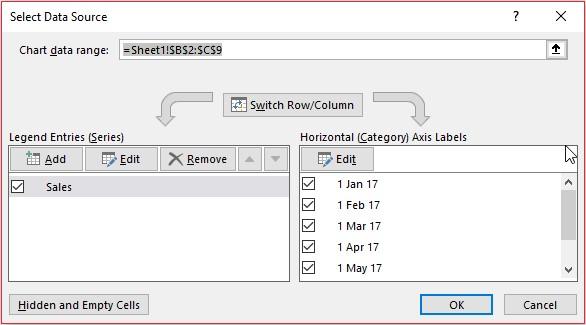
and from the resulting dialog box you update the date and sales references:

Surely there is a better way?  Oh yes – it’s dynamic range name time with a Table.

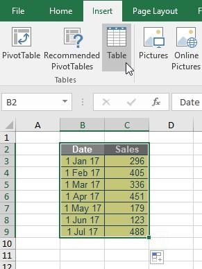
Let’s start again.  After entering the data and before creating the chart, convert the data range to a Table (CTRL + T, or from the ‘Insert’ tab on the Ribbon, choose ‘Table’ from the ‘Tables’ section):

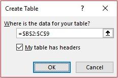
Ensure the ‘My table has headers’ check box is ticked in the ensuing dialog box:

Now add a chart as before, but this time, when additional data is added the chart automatically updates:

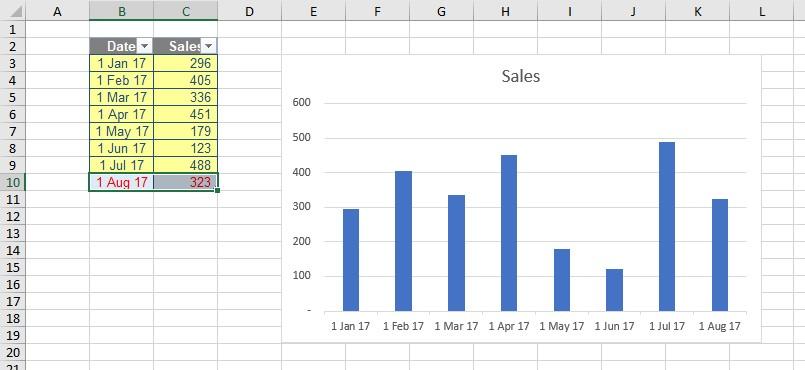
How good a trick is that?  Therefore, I have a rule with chart data: always put it in a Table before creating the chart.  It just makes life easier.

Tables can be used to make lists of variable length too.  Consider creating the following Table:

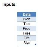
In this example, I will call this Table Table_List (I am nothing if not imaginative).  Selecting the range excluding the heading (‘Data’) is denoted Table_List[Data].  If I add further entries (e.g. “Devon” and “Hate” anyone?), the range Table_List[Data] will expand accordingly automatically.

I can create an in-cell list using data validation.  To do this, I go to the Ribbon and select ‘Data Validation’ from the ‘Data Tools’ group in the ‘Data’ tab of the Ribbon (keyboard shortcuts, either ALT + A + V + V or ALT + D + L):

The problem is if you make this the source of the data validated list,

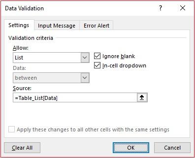
Excel doesn’t like it:

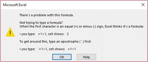
The type of formula used – structured referencing – is not compatible with source creation in data validated lists.  However, there is a simple workaround: just name this range, viz.

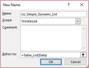
Here, I have named the range LU_Simple_Dynamic_List (LU simply stands for Look Up).  Now, if I use this as my source,

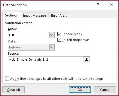
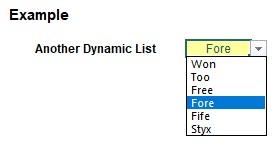
it works!  It’s a simple trick, but really useful and makes Tables one of your first ports of call should you require dynamic range names, e.g.

OFFSET Method

Sometimes, using the Tables approach is not appropriate.  Tables increase in depth when data is added, but what if the list should extend or contract based on a formulaic constraint?  Putting formulae in cells will automatically extend the Table, regardless if the outputs are seemingly blank (e.g. “”).

This method is older than the Table approach, as Tables only appeared as recently as Excel 2007.  The problem has been around for 20 years before that!  Hence, enter the OFFSET function.

The syntax for OFFSET is as follows:

The arguments in square brackets (Height and Width) may be omitted from the formula (they both have a default value of 1 which is explained further below). 

In its most basic form, OFFSET(Ref,x,y) will select a reference x rows down (-x would be x rows up) and y columns to the right (-y would be y columns to the left) of the reference Ref.  For example, consider the following grid:

OFFSET(A1,2,3) would take us two rows down and three columns across to cell D3.  Therefore, OFFSET(A1,2,3) equals 16, viz.

That’s how most people know – and use – OFFSET.  However, it is the Height and Width optional arguments that are the useful ones when it comes to dynamic range names. If we consider the extended formula OFFSET(D4,-1,-2,-2,3), it would take us first to cell B3 but then we would select a range based on the Height and Width parameters.  The Height would be two rows going up the sheet, with row 14 as the base (i.e. rows 13 and 14), and the Width would be three columns going from left to right, with column B as the base (i.e. columns B, C and D). 

Hence, OFFSET(D4,-1,-2,-2,3) would select the range B2:D3, viz.

Note that OFFSET(D4,-1,-2,-2,3) equates to #VALUE! since Excel cannot display a matrix in one cell, but it does recognise it.  However, if after typing in OFFSET(D4,-1,-2,-2,3) we press CTRL + SHIFT + ENTER, we turn the formula into an array formula: {OFFSET(D4,-1,-2,-2,3)} (do not type the braces in, they will appear automatically as part of the Excel syntax).  This gives a value of 8, which is the value in the top left-hand corner of the matrix, but Excel is storing more than that.  This can be seen as follows:

Indeed, we can construct a simple depreciation calculation, transpose references or even build a dynamic chart (one that displays more / less categories of information as required) using OFFSET’s Height and Width characteristics.  Let me demonstrate with a couple of examples (again, these are available for perusal in the attached Excel file). 

In the first example, consider the following ‘messy’ list:

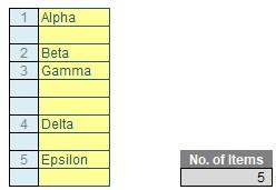
The number of items, given the range name No_of_Items, can be surmised simply using =COUNTA(Range), where Range is the data list (i.e. the cells in yellow).  COUNTA simply counts the number of non-empty cells in the Range.

Simple manipulation can create an interim list removing the spaces:

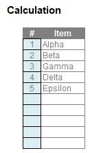
The aim is to make a list that does not include the five blank rows.  Assuming the first cell (i.e. where “Alpha” is situated) is cell F29 on the worksheet Sheet Name, we can define the list as

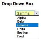
Note that the sheet name must be included in this formula for it to work.  No displacement occurs, but the depth is defined as five (No_of_Items) rows:

For the second example, just to change things up, I’ll use Width rather than Height.  Here, let’s consider chart data as follows:

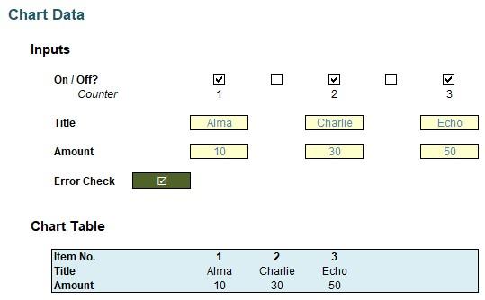
Check boxes have been used to include / exclude columns of data – in the example illustrated (above), only every other column is included (again, the Table methodology would not work directly here).  Simple manipulation gets the chart data table (highlighted in the blue box, above).

A standard chart would include five categories, two with blank names and null values, but very simply, I can produce the following chart instead:

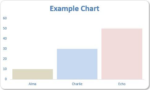
If I had four categories, the chart would update automatically to

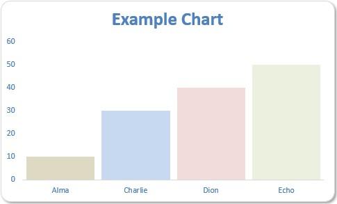
All we need to do is define the range for the amounts and data using OFFSET once more.  Assuming the chart data for titles starts in cell H25 of the SheetName worksheet, the formulae for the dynamic range names will be as follows:

LU_Dynamic_Amount:

LU_Dynamic_Title:

The width of these ranges will be MAX(SheetName!$H$24:$L$24), i.e. three in this instance.  This means the number of columns will total three!  This is why an error check is required here: if all cells are unchecked, there will be no chart to render.

To get the range names into the chart data, there is one more twist: the range names referenced must include the name of the workbook, e.g.

INDIRECT Method

Excel’s INDIRECT function allows the creation of a formula by referring to the contents of a cell, rather than the cell reference itself. 

The INDIRECT(ref_text,[a1]) function syntax has two arguments:

1. ref_text This is a required reference to a cell that contains an A1-style reference, an R1C1-style reference, a name defined as a reference, or a reference to a cell as a text string. If ref_text is not a valid cell reference, INDIRECT returns the #REF! error value.  If ref_text refers to another workbook (an external reference), the other workbook must be open. If the source workbook is not open, INDIRECT again returns the #REF! error value
2. [a1] This is optional (hence the square brackets) and represents a logical value that specifies what type of reference is contained in the cell ref_text.  If a1 is TRUE or omitted, ref_text is interpreted as an A1-style reference.  If a1 is FALSE, ref_text is interpreted as an R1C1-style reference.  Most modellers seldom consider this alternative referencing approach.

Essentially, INDIRECT works as follows:

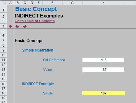
In the above example, the formula in cell H18 (the yellow cell) is

With only one argument in this function, INDIRECT assumes the A1 cell notation (e.g. the cell in the third row fourth column is cell D3).  Note that the value in cell H11 is H13, this formula returns the value / contents of cell H13, i.e. 187. 

This idea can be extended to consider data validated lists (again, this example can be found in the attached Excel file):

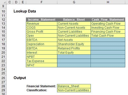
Here, I want to select a classification category in cell G29, based on the financial statement I select in cell G28 (e.g. Balance Sheet -> Non-Current Liabilities).

The trick here is not to include spaces in the names of the financial statements.  Then, in my illustration above, I have named cells F13:F23 Income_Statement, cells G13:G20 Balance Sheet and cells H13:H16 Cash_Flow_Statement.  Cells F12:H12 have been used to construct a data validation list in cell G28 and then the data validation list in cell G29 has used the INDIRECT function in the ‘Source:’ field as follows:

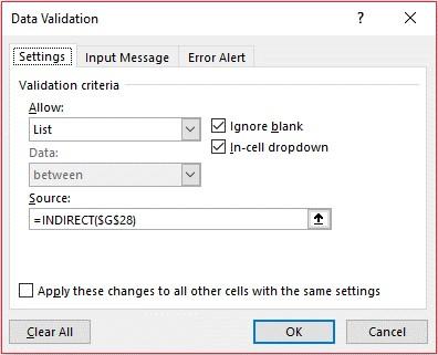
As a different financial statement is selected in cell G28, so the list will update in cell G29 (but only once the data validation list is activated, which is an Excel limitation).

IF Method

So what’s the most Important Function in Excel?  Any takers for IF?  The syntax for IF demonstrates just how useful this function is for financial modelling:

This function has three arguments: 

• logical_test: this is the “decider”, i.e. a test that results in a value of either TRUE or FALSE.  Strictly speaking, the logical_test tests whether something is TRUE; if not, it is FALSE
• value_if_TRUE: what to do if the logical_test is TRUE.  Note that you do not put square brackets around this argument!  This is just the Excel syntax for saying sometimes this argument is optional.  If this argument is indeed omitted, this argument will have a default value of TRUE
• value_if_FALSE: what to do if the logical_test is FALSE (strictly speaking, not TRUE).  If this argument is left blank, this argument will have a default value of FALSE.

This function is actually more efficient than it may look at first glance.  Whilst the logical_test is always evaluated, only one of the remaining two arguments is computed, depending upon whether the logical_test is TRUE or FALSE. 

This function lends itself to a switch or a condition that can be used to determine between two ranges, for example:

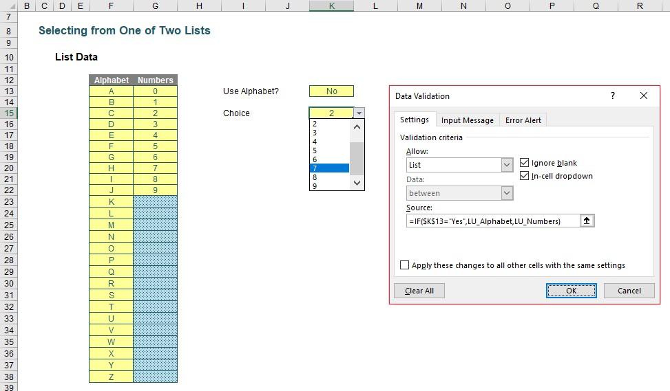
In this scenario, two range names have been set up: LU_Alphabet (cells $F$13:$F$38) and LU_Numbers (cells $G13:$G$22).  Cell K13 contains a Yes / No dropdown box which is used to determine which list is used to populate the in-cell list in K15. 

This latter cell uses data validation (ALT + D + L) with the source of the list defined as:

CHOOSE Method

Do you choose to use CHOOSE?  This function uses index_number to return a value from the list of value arguments.  CHOOSE may be used to select one of up to 254 values based on the index number (index_number).  

The CHOOSE function employs the following syntax to operate:

The CHOOSE function has the following arguments: 

• index_number: this is required and is used to specify which value argument is to be selected.  The argument index_number must be a number between 1 and 254, or a formula or reference to a cell containing a number between 1 and 254.
  • if index_number is 1, CHOOSE returns value1; if it is 2, CHOOSE returns value2 and so on
  • if index_number is less than 1 or greater than the number of the last value in the list, CHOOSE returns the #VALUE! error value
  • if index_number is a fraction, it is truncated to the lowest integer before being used.
• value1, value2, ...: value 1 is required, but subsequent values are optional.  There may be between 1 and 254 value arguments from which CHOOSE selects a value or an action to perform based on index_number.  The arguments can be numbers, cell references, defined names, formulas, functions, or text.

It should be further noted that:

• If index_number is an array, every value is evaluated when CHOOSE is evaluated
• The value arguments to CHOOSE can be range references as well as single values.

For example, the formula:

evaluates to:

which then returns a value based on the values in the range B1:B10.

The CHOOSE function is evaluated first, returning the reference B1:B10. The SUM function is then evaluated using B1:B10, the result of the CHOOSE function, as its argument.  A similar idea is also expressed by the formula:

which will return the result of =SUM(A1:A3).

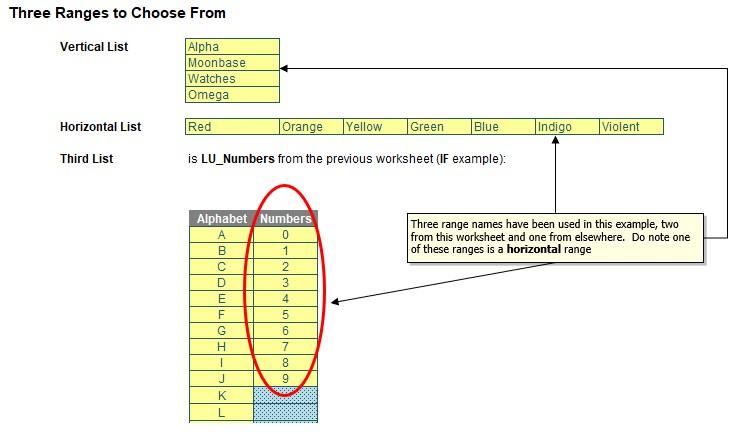
You may make the index_number a cell reference or formula which will therefore then choose from the selected list of ranges specified.  In essence, it’s like the IF example (above) but with more alternatives:

The attached Excel file provides an illustration of how this might work in practice.

Relative Referencing

By default, range names are referenced absolutely (i.e. contain the $ sign so that references remain static).  However, imagine a scenario where you are modelling revenue and you wish to grow the prior period value by inflation (already given a range name, say cell C3 on Sheet1).  Simply click on any cell (for example, I will use D17 arbitrarily), then define the new range name as follows:

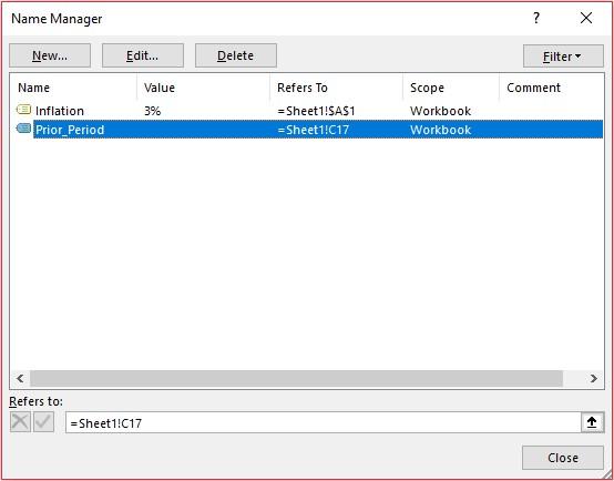
Note the ‘Refers to:’ entry.  Cell C17 (the cell to the left of D17) has been chosen without the dollar signs.  This is a relative reference.  Once we click on ‘OK’, the range name ‘Prior_Period’ will be defined as the cell immediately to the left of the active cell.  We can then inflate values easily by copying the formula

across the row, etc.

Word to the Wise

This article discusses just some of the methods available.  There’s a myriad of other functions that may be used, e.g. INDEX, COUNT and using arrays.  Further, data validated lists are used in many of the examples above.  Do remember that when data validation is based on a condition / criterion elsewhere, the data validation will not update until the data validated cell is edited next.

As you get more experienced, you’ll start to play – sometimes out of necessity.  That’s because Excel won’t always allow you to use dynamic range names in the same way “simple” range names may be used.  And there’s only one way to learn that: the hard way…