Using Styles Rather Than Formats in an Excel Workbook
This article highlights an Excel feature modellers might want to use more regularly. By Liam Bastick, director with SumProduct Pty Ltd.
Query
I’m competent in using Excel for my daily work, but I’d like to make the data more attractive and easier to read when I present it to other people in the business. Do you have any tips please?
Advice
Think about spreadsheets you have had to read or use. How easy has it been to find the key data or spot which cells should be changed to facilitate updated information? Have you ever noticed that spreadsheets built by colleagues look remarkably similar to your own and that they adhere to the company’s livery / branding / style requirements?
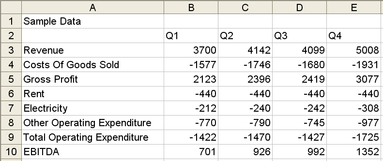
Not feeling comfortable with these questions? Rest assured, you’re far from alone.
Two key qualities of a good spreadsheet are consistency and transparency:
- Examples of Consistency:
- Formulae are copied without amendment across rows;
- Cells with a common purpose (e.g. inputs that are assumptions, such as inflation rates) are formatted similarly;
- Titles (e.g. sheet title, date headings) are positioned in the same cells in different worksheets;
- Assumption cells (i.e. containing data that may be changed by the user to affect model outputs) are unlocked, whereas all other cells are locked, so that in protected sheets / workbooks only these cells may be changed;
- Examples of Transparency:
- Assumptions are formatted to be instantly recognisable;
- Key outputs (e.g. totals) can be identified immediately, with their derivation obvious.
In the above illustration, using Excel’s Styles features can assist both transparency and consistency.
Formats and Styles
These terms are often used interchangeably, but ostensibly, they are not the same thing. To demonstrate, select any cell in Excel and apply the shortcut keystroke CTRL + 1. This shortcut brings up the Format Cells dialog box, viz.
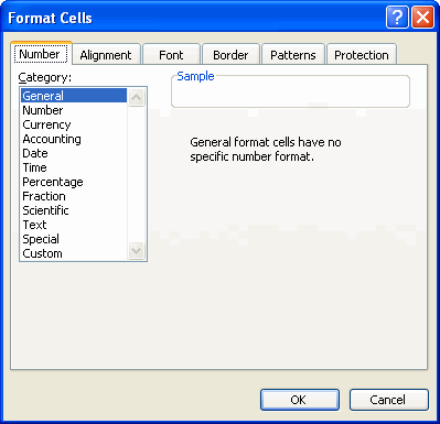
Excel has six format properties: Number, Alignment, Font, Border, Patterns and Protection. A style is simply a pre-defined set of these various formats. With a little forethought, these styles can be set up and applied to a worksheet cell or range very easily.
Creating your own styles is straightforward using Excel’s Style dialog box:
Excel 2003 and earlier
Go to Format–>Style(ALT + O + S):
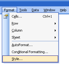
Excel 2007
Go to the Home tab and click the arrow in the bottom right corner and then select ‘New Cell Style…’ (ALT + N):

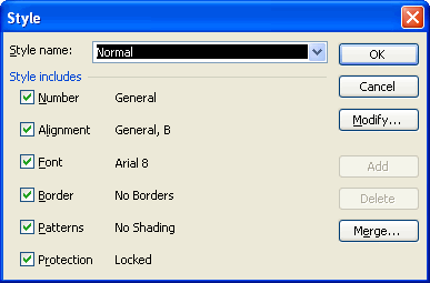
Either way, the dialog box appears, viz.
Example
We will create an assumption format for entering data in dollars. Firstly, select a cell or range of cells. Then, call up the above dialog box. The dropdown box (highlighted in the above figure) can be edited. We will change the name to “Dollar Assumptions” and click on the ‘Modify’ button (Excel 2002 and earlier) or the ‘Format’ button (Excel 2007).
The Format Cells dialog box reappears:
- Number: select the Currency category, with zero decimal places and apply the ‘$’ symbol;
- Alignment: Horizontal – Right (Indent) with zero indent;
- Patterns: select an ‘easy-on-the-eye’ colour such as pale green;
- Protection: uncheck the Locked check box (allows the cell to be changed in a protected worksheet);
- Click the ‘OK’ button to return to the Style dialog box.
Note that no formats have been ascribed for Font or Border in this example. We do not wish the style to control (i.e. overwrite) these properties, so the ‘Style includes’ check boxes for these two format properties should be unchecked:
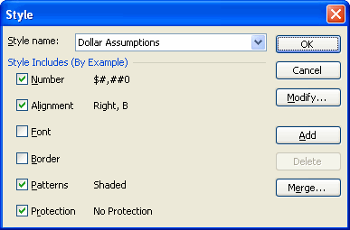
By clicking the ‘OK’ or ‘Add’ buttons, the cell or range has now been formatted with the ‘Dollar Assumptions’ style.
Now that this style has been added, in Excel 2007, you simply select the range and then click on the style in the Styles gallery on the Home tab. Applying styles in Excel 2003 (and earlier) is just as simple – once you have made a customisation.
For pre-Excel 2007, the standard way to apply a style is to call up the Style dialog box and then choose the appropriate style and click ‘OK’ – a little cumbersome. However, it is easy to incorporate this Style dropdown box on to an existing toolbar and dispense with several of these steps.
By right-clicking on any toolbar or using the shortcut (ALT + T + C + ENTER), call up the Customize dialog box and select the Commands tab, then the Format category.
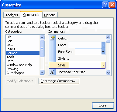
Choose the Style dropdown using the leftclick on the mouse and drag it onto an existing toolbar of your choice (then close the dialog box).

Easy!
Updating and Retaining Styles
The difference between Formats and Styles becomes obvious when you realise you want to change (update) a style. Simply select one of the cells that the style is attached to and then call up the Style dialog box in the usual way, modifying the style as required. Once finished click ‘OK’. Note that every cell in the open workbook that uses this style has been automatically updated. Once you start using styles, you will never look back!
You will only want to set up styles once. When finished, simply save the file as a template using File–>Save As (you may wish to delete / remove formatted cells first so that you have a ‘blank’ workbook). Using File–>New (or Office Menu–>New–>My Templates… in Excel 2007) will call up your saved styles in moments.
Styles – Before and After
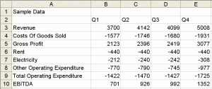
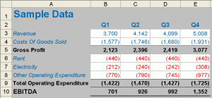
Returning to our original query, which do you prefer?
Before Styles
After Styles
If you have a query for this section, please feel free to drop Liam a line at liam.bastick@sumproduct.com or visit the website www.sumproduct.com

