Finding Your Perfect Match
Here, we consider how to undertake a case sensitive match. By Liam Bastick, Director with SumProduct Pty Ltd.
Query
I am trying to sum data based on case sensitive criterion and cannot get Excel to distinguish between upper and lower case characters, which is resulting in incorrect results. Any suggestions?
Advice
This is quite a common question over the years causing problems for many. To illustrate the issue, consider the following example which comes from the attached Excel file:
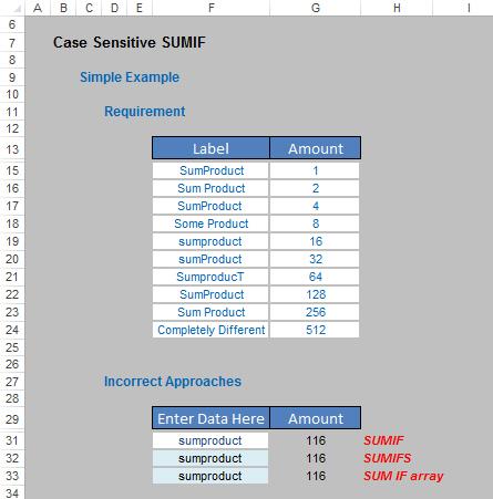
Various text strings in cells F15:F24 have been allocated corresponding values in cells G15:G24. The numbers have been chosen deliberately so that it is clear which rows have been included in the overall total.
We have discussed working with criteria before (see Dealing with Multiple Criteria and SUMPRODUCT Squared..?). Unfortunately, it is clear to the eye that only row 19 contains “sumproduct” and so the results for looking up “sumproduct” in the table should be just 16 and not 116 as returned presently.
To circumvent these problems, we consider a combination of two functions.
Remembering an old friend: SUMPRODUCT
Imagine we are presented with the following sales report:
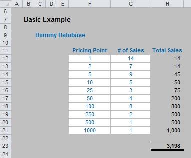
The sales in column H are simply the product of columns F and G, e.g. the formula in cell H12 is simply =F12*G12. Then, to calculate the entire amount cell H23 sums column H. This could all be performed much quicker using the following formula:
=SUMPRODUCT(F12:F21,G12:G21)
i.e. SUMPRODUCT does exactly what it says on the tin: it sums the individual products.

Dealing with Multiple Criteria
Where SUMPRODUCT comes into its own is when dealing with multiple criteria. This is done by considering the properties of TRUE and FALSE in Excel, namely:
- TRUE*number = number (e.g. TRUE*7 = 7); and
- FALSE*number = 0 (e.g. FALSE*7=0).
Consider the following example:
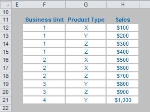
we can test columns F and G to check whether they equal our required values. SUMPRODUCT could be used as follows to sum only sales made by Business Unit 1 for Product Z, viz.
=SUMPRODUCT((F12:F21=1)*(G12:G21=”Z”)*H12:H21).
For the purposes of this calculation, (F12:F21=1) replaces the contents of cells F12:F21 with either TRUE or FALSE depending on whether the value contained in each cell equals 1 or not. The brackets are required to force Excel to compute this first before cross-multiplying.
Similarly, (G12:G21=”Z”) replaces the contents of cells G12:G21 with either TRUE or FALSE depending on whether the value “Z” is contained in each cell.
Therefore, the only time cells H12:H21 will be summed is when the corresponding cell in the arrays F12:F21 and G12:G21 are both TRUE, then you will get TRUE*TRUE*number, which equals the said number.
Meet a new friend: introducing the EXACT function
EXACT is a function we haven’t discussed previously. Its syntax is as follows:
=EXACT(Text1,Text2)
This function compares two text strings and returns TRUE if they are exactly the same, FALSE otherwise. It should be noted that EXACT is case-sensitive but ignores formatting differences.
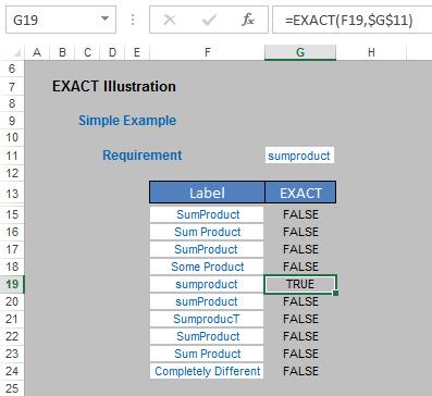
Using our original example, EXACT is very simple to understand: either something is precisely the same or it is not.
Having brought these two functions into sharp focus, the suggested answer should be imminently obvious.
Suggested solution
The suggested solution to our problem is just a combination of these two functions, viz.
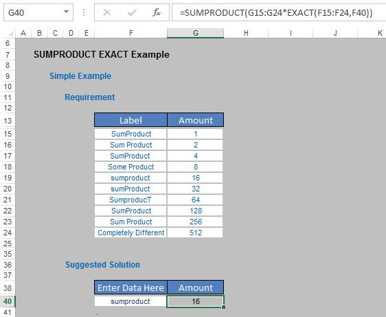
The suggested solution is
=SUMPRODUCT(G15:G24*EXACT(F15:F24,F40)).
which simply includes only values that precisely match the value typed in cell F40. The attached Excel file demonstrates a similar solution.

