Identifying Links

Sometimes deliberate and sometimes inadvertent, external links often work their way into our Excel workbooks. To understand what they are, where they are and why they exist, we need to first know which external sources are referenced, because we can’t find what we are looking for if we don’t know what we are looking for. I feel a U2 song coming on. That’s right, I can’t live with or without my links – of which there may be more than One [please stop – Ed.].
Many years ago, I wrote an article that explained how a macro could be employed to list all external links in an Excel workbook:
Sub ListExternalLinks()
Dim ws As Worksheet, TargetWS As Worksheet, SourceWB As Workbook
If ActiveWorkbook Is Nothing Then Exit Sub
Application.ScreenUpdating = False
With ActiveWorkbook
On Error Resume Next
Set TargetWS = .Worksheets.Add(Before:=.Worksheets(1))
If TargetWS Is Nothing Then ' the workbook is protected
Set SourceWB = ActiveWorkbook
Set TargetWS = Workbooks.Add.Worksheets(1)
SourceWB.Activate
Set SourceWB = Nothing
End If
With TargetWS
.Range("A1").Formula = "Link No."
.Range("B1").Formula = "Cell"
.Range("C1").Formula = "Formula"
.Range("A1:C1").Font.Bold = True
End With
For Each ws In .Worksheets
If Not ws Is TargetWS Then
ListLinksInWS ws, TargetWS
End If
Next ws
Set ws = Nothing
End With
With TargetWS
.Parent.Activate
.Activate
.Columns("A:C").AutoFit
On Error Resume Next
.Name = "Link List"
On Error GoTo 0
End With
Set TargetWS = Nothing
Application.ScreenUpdating = True
End Sub
Private Sub ListLinksInWS(ws As Worksheet, TargetWS As Worksheet)
Dim cl As Range, cFormula As String, tRow As Long
If ws Is Nothing Then Exit Sub
If TargetWS Is Nothing Then Exit Sub
Application.StatusBar = "Finding external formula references in " & _
ws.Name & "..."
For Each cl In ws.UsedRange
cFormula = cl.Formula
If Len(cFormula) > 0 Then
If Left$(cFormula, 1) = "=" Then
If InStr(cFormula, "[") > 1 Then
With TargetWS
tRow = .Range("A" & .Rows.Count).End(xlUp).Row + 1
.Range("A" & tRow).Formula = tRow - 1
.Range("B" & tRow).Formula = ws.Name & "!" & _
cl.Address(False, False, xlA1)
.Range("C" & tRow).Formula = "'" & cFormula
End With
End If
End If
End If
Next cl
Set cl = Nothing
Application.StatusBar = False
End Sub
If you are terrified of VBA and hate programming, don’t worry – feel free to ignore the above: I have no plans to explain it. I reproduce it for effect only.
Whilst working on a client project recently, I came across this wonderful trick that combines old, “outdated” Excel with one of the very latest features in Excel. It is so simple and just blows the above solution out of the water. I would love to take the credit for this, but I cannot: long-time Excel Most Valuable Professional (MVP) Bob Umlas, please take a bow, because the crux of this trick belongs to you.
Before Visual Basic for Applications (VBA) came to Excel, coding was undertaken using what were known as Excel 4.0 (“xl4”) macro functions. These old xl4 macro functions are still doing the rounds because Microsoft cannot get rid of anything, because the software giant knows some spreadsheets still in use were developed probably before the wheel was.
I have written about EVALUATE before, which is a very useful function (it essentially converts text strings into formulae that may be, er, evaluated). For example, consider the following complex spreadsheet:

Theoretically,
=EVALUATE(A1&A2&A3)
would be EVALUATE(1+2) which is 3. That’s all good, except it doesn’t work unless you use it via a range name definition.
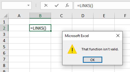
You won’t find it in Excel Help (“That function isn’t valid.”), but as I say, it is recognised as long as you use it inside an Excel range name. And its sister function, LINKS, which recognises external links in an Excel workbook, behaves very similarly.
The process for identifying and listing your links in an Excel workbook is very easy.
First, let’s define a range name. I can do this using ‘Defined Name’ in the Formulas tab of the Ribbon:

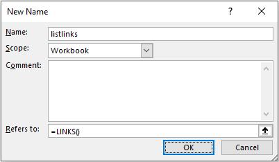
This calls the ‘New Name’ dialog:

Here, I have created a new range name, called listlinks, which refers to the formula
=LINKS()
If I were to type this formula straight into a cell, I would get the following (aforementioned) error:

but that’s sort of untrue indirectly. If instead I were to type in =listlinks (i.e. my freshly minted range name), I wouldn’t get an error if the model contains external links and you have an Office 365 version of Excel:

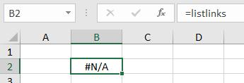
However, if the model doesn’t contain links, I would receive a prima facie error:

In the first instance, Office 365 has spilled the references, i.e. it has listed the references in adjacent cells along the same row. Good old Excel: it does like to default on the incorrect choice. To counter this great default “feature”, if I were to use TRANSPOSE, suddenly things become much more readable:

Voila! All your links presented dynamically.
This is just so much simpler than convoluted VBA code or using third party software. All you need is the ability to spill your results, i.e. your version of Excel supports dynamic arrays (presently, this means using an Office 365 version of Excel).
That’s all there is to it.
Word to the Wise
Excel 4.0 functions stored in defined names may only be saved in macro-enabled workbooks (.xlsm or .xlsb). If using this feature in conjunction with dynamic arrays, the file will have to be generated using Excel 365 too, so do be aware of these limitations when incorporating this functionality into existing workbooks.

