Rolling Budgets

This article considers a simple approach to maintaining rolling budgets / forecasts in Excel. By Liam Bastick, director with SumProduct Pty Ltd.

Query

What is the best way to put together a rolling budget in Excel?

Advice

Depending upon where the fiscal year ends, the start of a new calendar year can mean revisiting the old budgeting / forecasting spreadsheet to either revisit the assumptions and / or tweak the start date.

One popular forecasting tool is the so-called “rolling budget” whereby a certain period of time is forecast (e.g. next six / 12 / 18 months) starting from a particular date, which may be varied. To allow for this flexibility, less experienced modellers will manage this by copying and pasting assumptions from later periods to earlier periods. Even less experienced modellers may cut and paste the same data, which can result in model formulae becoming severely compromised. Both methods are fraught with dangers.

We suggest a more robust – and flexible – technique instead.

Imagine you have the following set of assumptions:

In this very simple illustration, you wish to calculate gross profit for a particular six months, say starting from April. The first thing you do is leave this input page alone!

Instead, you set up an interim calculations page as follows:

In this example, cell D3 is an input cell, which could actually be data validated as a drop down list (see >Controlling Your Inputs for further details):

The formula in row 5 is based on this input (hopefully that calculation is straightforward) and then we use the OFFSET function (see Onset of OFFSET for further details) to create similar calculations in rows 6, 8 and 10 (although row 10 is then multiplied by row 8’s values also).
For example, the formula for Sales in cell D8 is simply:

The idea is incredibly simple but very powerful. Inputs from previous periods can be retained and because a range of data has not been specified, periods can be added to both the inputs and calculated pages to allow for other start dates and longer forecast periods, etc.

Including Actual Data

When actual data is input into a model, frequently it replaces the original information, and therefore management loses the ability to see how accurate forecasts were originally and how budgeting may be improved.

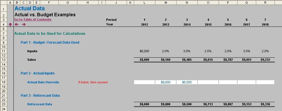
One way round this would be to simply incorporate “Actuals” into the future forecasts. For example, we may wish to undertake variance analysis by comparing actual data with the original budgeted information. In this case, we would suggest the following approach:

Rows 9 to 13 of this illustration simply reiterate the calculations already detailed above regarding the original forecasting.

Note row 18 however: this is where actual data is added instead. In this example, we simply use hard coded inputs for the data, but it only requires a simple variation to this methodology to revise growth rates, etc.

Inputs are added wherever updated data (e.g. actuals) is available; otherwise we fall back on the original data and calculations. This is achieved by the formula in row 23 in my example, which is (for cell L23):

i.e. if there is data in the corresponding cell in row 18 use it; if not, if it is the first period take the original input value, otherwise simply inflate the prior period amount by (1 + growth) rate for that period. It may include a nested IF statement, but it is still a relatively simple and straightforward calculation.

For more on Actual versus Budget issues, please see Modelling Actual versus Budget.

Error Estimates

Where actual data and projections are used, variance analysis surely follows. In order to ascertain how well we have forecast we often use measures that estimate bias and accuracy:

• Bias – A forecast is biased if it errs more in one direction than in the other (i.e. we under-estimate or over-estimate on a regular basis)
• Accuracy – Refers to the distance of the forecasts from the actual data, ignoring the direction of that error,

The idea here is that forecasting is an iterative technique and we use the outcomes from our error analysis to refine our forecasting techniques (e.g. not using all of the historical data, making “normalising adjustments”).

Consider the following example. For six time periods, t₁ to t₆, we compare actual demand at time t, D_t, with forecast demand at time t, F_t, as follows:

Obviously, this is not enough data points to make a proper conclusion – the intention here is merely to provide an illustrative example.

We can consider the following measures:

• Cumulative sum of Forecast Errors (CFE). This measures both bias and accuracy, SUM(Et) = -20
• Mean Absolute Deviation (MAD). This considers the magnitude of the average error, 170 / 6 = 23.33
• Mean Squared Error (MSE). An alternative to MAD, it takes the square of the errors and divides it by the number of observations, 5,150 / 6 = 858.33
• Standard Deviation (SD). A common technique to measure the ‘spread’ of the distribution, care needs to be taken if the error spread is skewed in one direction or another (e.g. if the magnitude of CFE is large), SQRT(MSE) = SQRT(5,150 / 6) = 29.30 [this may be divided by one less than the size of the sample by statisticians]
• Mean Absolute Percentage Error (MAPE). This is the average of the percentage errors, 83.49% / 6 = 13.91%.

No one technique should be used in isolation, although the Standard Deviation (SD) approach is perhaps the one most commonly employed.

Examples of all of the above may be found in this attached Excel file.