Taking Stock of Inventory

Query

How do I calculate movements in inventory and associated costs of goods sold (COGS) in my financial model so that my financial statements balance / reconcile?

Advice

The aim of this article is to provide a concept by using a walkthrough model.  Therefore, please refer to the attached Excel file.  Using this example, I will run through a step by step process that will detail how to construct an integrated model forecasting the flow of inventory.

In this example, the model assumes that money is received on credit sales (days receivable) 60 days after the sale is made and that bills / creditors are paid 30 days after the invoices have been received (i.e. days payable is 30) for all periods.

I am going to need some further assumptions:

The first task is to imagine that you have the assumptions above, and now you have to model the sales and correctly insert those amounts into your financial statements accordingly.  This has to be calculated first as this has knock-on effects on costs of sales (COGS) and hence inventory.

Therefore, I will create a Revenue segment where we pull the relevant data to calculate the sales:

Notice that when I first create a calculations section I simply refer to assumptions from elsewhere, rather than perform calculations on these figures at the same time.  This makes it easier for end users to follow model logic. 

Next, I have calculated the price per unit from the initial unit price, and then adjust for inflation each period.  The projected sales amounts are pulled directly from the Assumptions projected sales row 26 in the example file:

The Days Receivable section pulls the assumptions from row 51, then calculates the Closing Receivables. The Closing Receivables is a simple formula that multiplies the amount received by the fraction 60 / 365 (if not a leap year) to calculate the amount that is still due at the end of year.  Essentially, this assumes that all of the payments are distributed evenly throughout the year.

Knowing the sales for the period and the receivable for all periods, I can construct the control account, where the opening / closing receivables and revenue are linked directly from the calculations above.  We have three of the four lines for the account: the Cash Receipts is then simply balancing figure:

Now that revenue has been computed, we can move on to considering the inventory account itself.  This comprises two key movements: additions (the purchases of stock made) and deductions (both wastage and the stock used for sales – the latter is why I had to calculate sales first).  

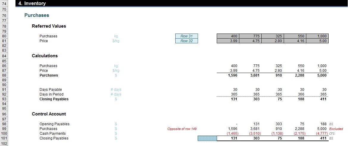
Again, I have cited the necessary data from the Assumptions section, which comprises of the Purchases and Price data:

The calculations for Payables are relatively straightforward, with the Purchases being the product of the Purchases made and the Price.  The Closing Payables formula is similar to the Closing Receivables formula (above):

As before, this assumes that the payments for the products are distributed evenly throughout the year.

Now, I must create the control account here, Opening Payables linked to the blank cell, to ensure that the previous period is taken into account.  The Purchases reference row 88, the Closing Payables reference row 93, hence the Cash Payments are the balancing figures. 

But that’s not the end of the calculations.  The calculations in this section get a little complicated now.  Bear with me though as it will all make sense in the end…

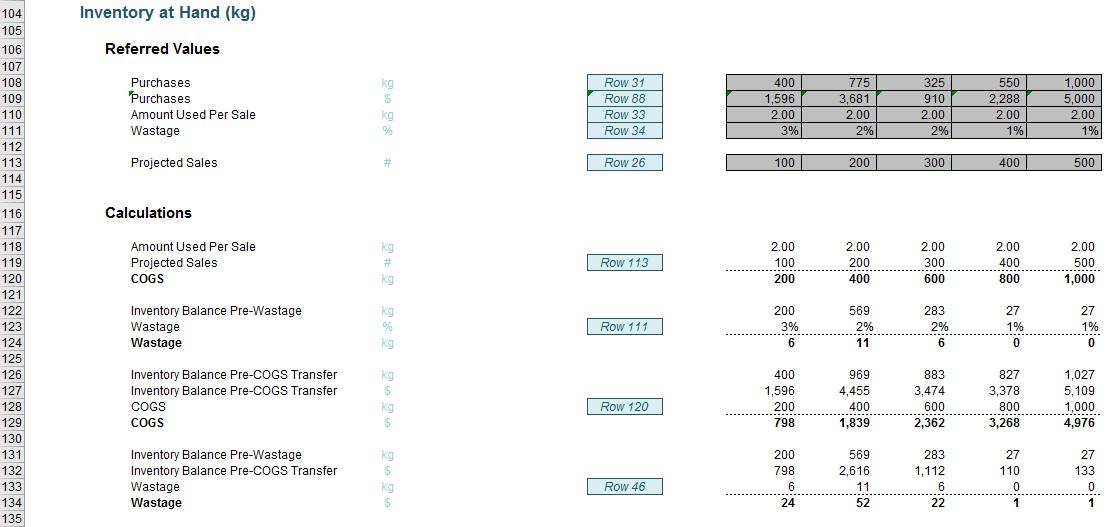
There are two COGS calculations to be made here: the first concerns weight and the second concerns pricing.  We need to separate the two since we need the weight of the COGS to help work out the inventory amounts, in order to ascertain pricing.

The Amount Used Per Sale (row 118), Projected Sales (row 119) and the COGS (row 120) are relatively straightforward, with COGS just being the product of the two earlier rows.

Moving on to the Inventory Balance Pre-Wastage (row 122), this row is calculated from the sum of the Opening Inventory, Purchases and the COGS (rows 139 to 141). This is so that the later calculations will take the previous period into account, as the Opening Inventory line draws figures from the previous periods. 

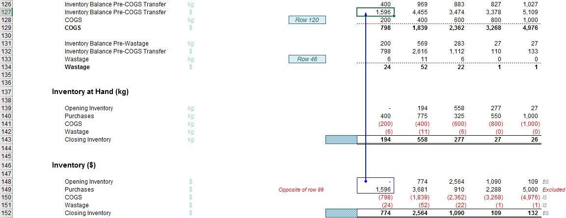
The Inventory Balance Pre-COGS Transfer (row 126) is calculated from the Opening Inventory and Purchases from the Inventory at Hand (kg) section (rows 139 and140):

The next line down may appear to be the same, but notice the units, delineating that the input should be a dollar figure.  Thus this figure is calculated from the sum of the Opening Inventory and the Purchases rows (rows 148 and 149) in the Inventory ($) section:

An IF statement that calculates the dollar value of the COGS:

i.e. this IF statement states that if there is a non-zero weight for Inventory Balance Pre-COGS Transfer, calculate the dollar amount of this balance multiplied by the proportion of the COGS weight divided by the Inventory Balance Pre-COGS Transfer (essentially the proportion of units left).  So, if COGS is 200, means 200 units have been sold, so there are 400 – 200 = 200 units left.  Therefore, I multiply the total value of the stock on hand 1,596 by 200 / 400, which is 798 (row 132):

Wastage is calculated simply by referencing the relevant inputs.  Inventory Balance Pre-Wastage (kg) is just the Inventory Balance Pre-COGS Transfer (kg) less COGS (kg) (rows 126 and 128), and the Inventory Balance Pre-COGS Transfer ($) is just the Inventory Balance Pre-COGS Transfer ($) less then COGS ($) (rows 127 and 129).

The wastage formula is very much like the COGS calculation above:

It’s now just a matter of calculating the control accounts for inventory, both in terms of weight and costs.

The opening inventory line has to be linked to the previous period’s closing.  This ensures that the closing balance of the previous period is taken into account.  The purchases are linked from row 108.  The Wastage and COGS amounts are pulled from the previous calculations, row 134 and 120 respectively.  You should remember to negate these two cell references: 

The same steps are repeated with the Inventory ($) section, just note the difference in references to match the unit ($):

So will it balance?  Do you think I’d have written this article if it didn’t?

Notice the indiscreet ‘BS’, ‘IS’, and ‘CF’s scattered about the model?  They are not there merely for aesthetic purposes: they are the control account line items to be entered into the financial statements, viz.

There’s no tricks here, just a simple linking of all of those lines to the respective finanical statement segment.  Do note the two “Excluded” line items (rows 99 and 149 in the example): they will always be equal and opposite so may safely be ignored. 

Furthermore, if you inspect the attached Excel File you will see that row 171 has this formula to calculate cash:

Anchoring column J allows the formula to provide a running total.  Also note a similar formula is used in the Bank Overdraft row:

This just ensures positive cash balances are displayed as Cash whilst negative running totals are displayed as an Overdraft.

Word to the Wise

This example calculates COGS on a weighted average basis.  Other techniques include Last In, First Out (LIFO) and First In, First Out (FIFO).  This requires more involved calculations using a grid system similar to the calculations performed in a depreciation calculation (see this Depreciation article for further details).  However, once the costs have been computed, the rest of the method is similar to the approach described above.