Dependent Data Validation lists for many sets of input cells
Drop-down lists in Excel are good, but we have a tip to make them much better!
Using Data Validation (DV) to create a drop-down list in a cell makes your spreadsheet easier to use and it keeps the data valid, hence the name. To take it further, we’ll show you how to set up drop-downs that work with each other so each one will filter what can be selected in the next (dependent drop-downs). We don’t stop there. We’ll also show how to apply one set of dependent lists to as many input cells as needed! We think this is very powerful. If you already know how to make dependent DV drop-down lists, you can skip ahead, otherwise we’ll explain how that works so you have a good foundation about basic DV drop-down lists and how to make one dependent on another.
To follow along, you can download our Excel file.
Dependent Data Validation
In Excel, you can set up one drop-down list to make data entry easy or to limit what can be entered in a cell. With a little more work, you can set up 2 drop-downs such that the values in the 2nd list depend on the value chosen in the 1st. You can add a 3rd drop-down that depends on the values chosen in the first 2, and so on. This can make data entry a lot easier for someone using the spreadsheet. Let’s say you have a long list of products. You can make it easier to find a product by grouping them into product categories and setting up a drop-down to select the category first. Then use up a drop-down that shows only the products for the selected category.
As we show in the screen shot below, “coffee maker” was selected in the Category column, and then the drop-down in the Product column shows only coffee makers. After selecting a coffee maker, the drop-down in the Color column will show only colors for that coffee maker.
Keep reading and you’ll learn how to set up the drop-downs for an entire table with as many rows as you need.

A basic Data Validation drop-down list
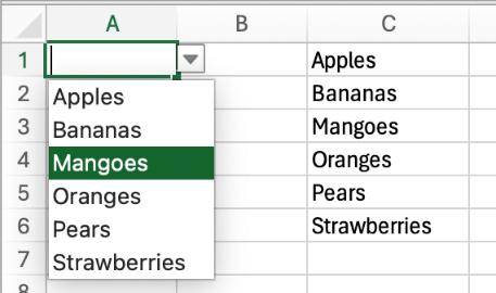
Let’s start with the basic building blocks. To make a simple DV drop-down list, you can enter a list of values in a few cells, then set a DV rule that refers to the list, as in the example shown below. We have various fruit listed in cells C1:C6, and we create a DV rule allowing a “List” with that range as the source. In the cell where we apply the rule, a drop-down appears so you can pick from the list rather than typing.
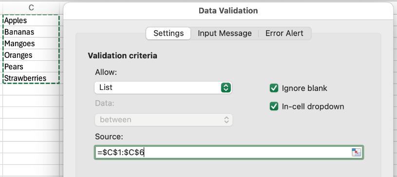
Simple as that, you now have a drop-down with all the types of fruit, making it easy to select, but preventing wrong values from being entered.
How to make one drop-down dependent on another
It’s straightforward to create a drop-down list that depends on the value of a selection in another drop-down list.
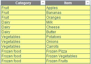
Put your data into a table with 2 columns. As an example, you might have a list of categories and items. If you pick a category, the drop-down will show items for that category. The example shown here has categories and specific food items.
Then choose a cell with empty rows below it and enter a formula to get the unique values from the first column of your table. For example, we could use:
=UNIQUE(tblFoods[Category])
for a table called “tblFoods”. You need to have empty rows below your formula, because it will spill into multiple rows. If there aren’t enough empty cells, you’ll get a #SPILL! error. In our sample file, we put this formula in F38 on the sheet called “Basic Dpdnt DV”.
As a tip, it can be useful to sort the values by using the SORT function, e.g.:
=SORT(UNIQUE(tblFoods[Category]))
In this example, the formula gets the unique categories for foods you might buy at a grocery store.
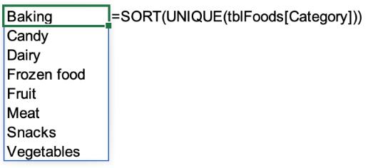
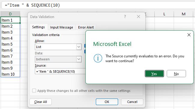
NOTE: Since we’re going to turn this list into a Data Validation drop-down, why don’t we just write the formula into the Data Validation rule? As of this writing, Excel will not accept a dynamic array formula directly in the Data Validation dialog. In the example shown below, the formula ="Item " & SEQUENCE(10) will generate a list of values like “Item 1”, “Item 2”, etc. in the sheet. If you use that same formula as the source for a DV drop-down, Excel will show an error saying “The Source currently evaluates to an error. Do you want to continue?”. If you choose Yes, then the drop-down won’t show any values.
Go to the Name
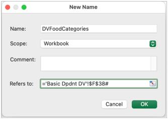
Manager and create a new named item referring to the cell that contains the
formula, and make sure you put “#” at the end so that it will include all the
values that spill from that cell. For
example, you might have a name such as DVFoodCategories and set the “Refers To”
field to =$F$38# if your formula is
in cell F38, as in our example file.
Select the cell
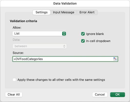
where you want the Categories drop-down list to appear, go to Data > Data
Validation, and enter the following options:
- Allow: List
- Source: =DVFoodCategories (Tip: To enter the Name in the Source field, just press F3 and choose it from the list that pops up).
Let’s
say you created the drop-down in cell F14. Now you need to create a drop-down list for
the Items. To do this, go to another
cell with empty rows below it (G38 in our sample) and enter the formula to get
all the Items from your table that have the category selected in F14. It’s similar to the formula for the categories
(F38), but you need to filter the list. The FILTER function is perfect for this.
We can use the following formula:
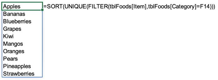
=SORT(UNIQUE(FILTER(tblFoods[Item],tblFoods[Category]=F14)))
This creates a list of Items from tblFoods that have the Category selected from the drop-down in F14.
Then create a Name such as “DVFoodItems” that
refers to $G$38.
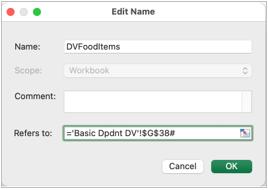
Then select the
cell where you want the drop-down and set a DV rule with Allow: List and
Source: =DVFoodItems
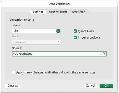
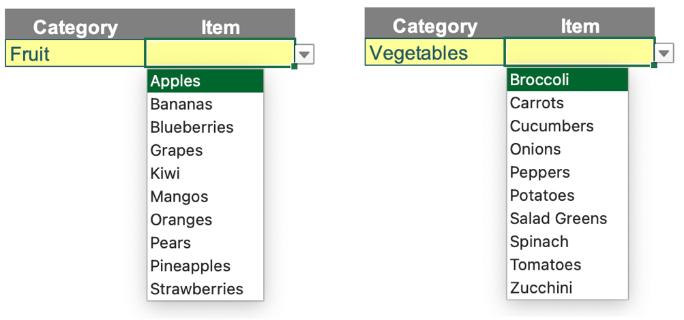
When you pick a category from the first drop-down (F14), the drop-down in G14 will only show choices from that category, as shown in the following images:
How do you make this scalable?
Let’s say you want to make an order form, where you can pick up to 10 items. Does it mean you need to set up a data validation list for each row? You wouldn’t need to do that for Categories, because you’d use the same category list for all 10 rows. But the Item lists can be different on each row. You could create a filtered item list for row 1 as we showed in the example above, then create a similar list for the category selected in row 2, then row 3, and so on. To pick items on 10 rows, it seems like you would need to set up 10 formulae to create the item lists, such as DVFoodItemsRow1, DVFoodItemsRow2, etc.
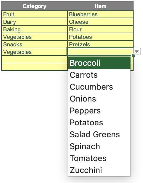
Using the steps we mentioned earlier, each row would need a formula to filter its items, referring to the category cell on the row. However, we don’t want to tediously repeat the setup for each row.
Fortunately, there’s a solution that lets you create one formula to do the job for any number of rows where you want to use a drop-down to choose the Item.
The CELL is the key
Excel has a function called CELL that you can use to get information about a cell, such as the address, row, column and a few other things. For example, the formula:
=CELL(“address”, A1)
will give you the result “$A$1”. That might not seem terribly useful, because you already know the address of A1. It’s just giving it to you in text form.

Despite how underwhelming the CELL function may initially seem, it’s actually very useful. It’s the key to making our drop-down lists work while avoiding lots of repetitive setup work. One of the unique things about the CELL function is that if you don’t provide a cell reference to it, it will give you information about the cell that was active when Excel last recalculated. It’s sort of saying “if you don’t tell me which cell to look at, I’ll just look at the last cell you looked at.”
If you omit the cell reference from the example above, =CELL(“address”), it shows its special effect. Rather than always giving the same result, the value will change depending on the last active cell when Excel recalculated. In the example shown here, we have just entered “hello world” into C1. Each time we enter a value, Excel recalculates. It shows the address $C$1, since that was the active cell when Excel last recalculated.

Do you see where we’re headed with this solution? We can use the CELL function to dynamically find the last category that was selected on any row! In our formula that gets the Items list for the category that’s been selected, we don’t need to refer to a specific cell. We can make the Items drop-down show the items for whatever category was just chosen, across all rows.
In the example here, we’ve set up a table to enter multiple categories and items, and it uses the same DV rule for all the drop-downs in the Item column. It adjusts accordingly when you pick a Category on any of the rows.
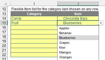
Let’s see how to set that up. If you know the trick about using the CELL function, it’s straightforward. You can create a formula that will get the last chosen category, no matter which row it’s on.
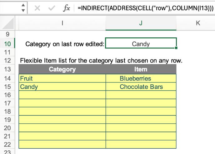
In our example below, the formula in J10 is:
=INDIRECT(ADDRESS(CELL("row"),COLUMN(I13)))
We use ADDRESS(CELL("row") to get the row of the last edited cell, which is row 15. We use COLUMN(I13) to get the column number for Category, which is column 9. So it’s calculated as INDIRECT(15, 9), which gives the value “Candy” which is in cell I15 (row 15, col 9).
Then, we just need to create a formula
to get the Items for the current category. In the example below, the value for the
category is in J35. In this case it’s
getting all the items for the “Candy” category.
The formula is:
=SORT(UNIQUE(FILTER(tblFoods[Item],tblFoods[Category]=J35,"Pick a category first.")))
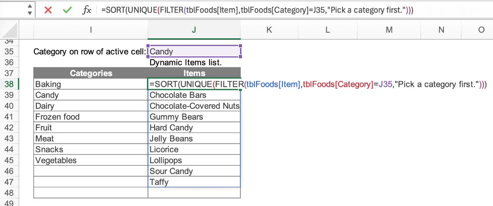
Let’s break it down:
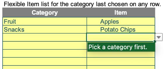
- We use FILTER(tblFoods[Item],tblFoods[Category]=J35,"Pick a category first.") to get the list of items from our table with the category found in J35. The last argument is "Pick a category first.", which will show up if there are no matching Items. If you try to select an Item without having picked a Category in that row, the drop-down will show “Pick a category first.”
- We use the UNIQUE function to make sure there are no duplicate items, and SORT to put them in order.
Now that we have our list of Items in cell J38, we can create a Named Range to easily refer to it in our DV rule. Just create a name referring to J38#. The # is very important, because it will include all the items that spill from J38. Without it, the drop-down will only show the first item in the list.
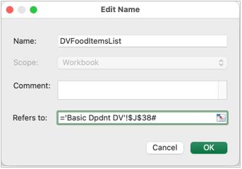
Next, we can apply the DV rule to all
the cells in the Item column of our table - one rule for all.
Select all the cells in the Item column, and press Data > Data Validation.
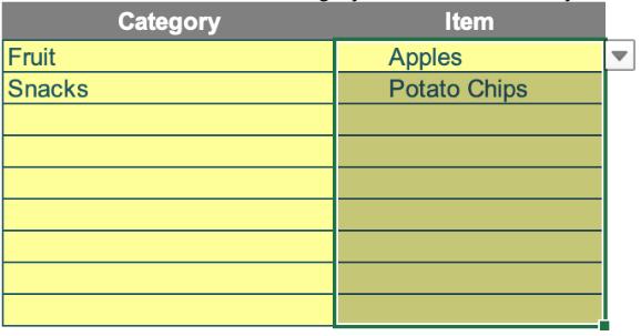
Set “Allow” to List, and set the
Source to =DVFoodItemsList. Press OK and you’re ready to see it in action.
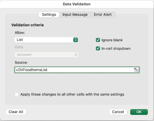
To test it out, try the following:
- Pick a category in any row, then pick an item in the same row.
- Try to pick an Item in a row where you haven’t picked the Category. The drop-down should show “Pick the category first.” as the only choice.
- Pick a category in any row, then pick an item in a different row. This is where it may run into a problem. The list of items will be for the last category that was picked, which may not be a match if you try to pick an item on a different row. We have a solution for this, too. Keep reading
Don’t allow the same item twice
An option for the Items drop-down is to add a secondary filter to reduce the drop-down choices to only items that we haven’t already chosen in our list. In the example below, we show that most of the 'Baking' items have already been added to our table. The drop-down only shows the remaining few items. If we select 'Chocolate Chips' and then re-open the drop-down, 'Chocolate Chips' are no longer available to select. If we then select 'Baking Soda', 'Chocolate Chips' are on the drop-down again.
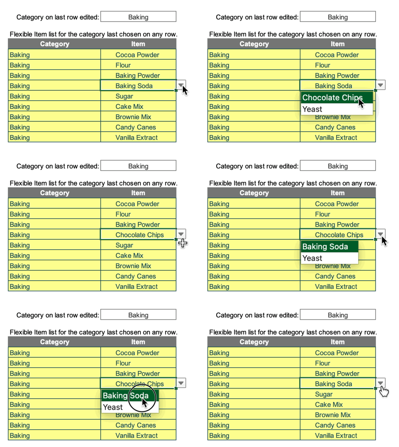
To make this work, we need to add a filter to the formula that generates the list of items. The formula below does that for us. You can see this formula in L38 of the sample file.
=LET(AllowUsed,FALSE,items,SORT(UNIQUE(FILTER(tblFoods[Item],tblFoods[Category]=J10,"Pick a category first."))),IF(AllowUsed,items,FILTER(items,ISNA(XMATCH(items,J14:J22,0)))))
We used the LET function to make it shorter and more readable. Let’s break this one down.
- The first name is AllowUsed, and we give it a value of FALSE. We’ll use this later, but the important point is that you can change FALSE to TRUE switch the list to allow items that have already been selected.
- The next name is items, and we give it a value that is all the foods for the given category. It’s the same as the formula we discussed in the previous section.
- Next we have our calculation. If AllowUsed is TRUE, then it uses items with no additional filter. If AllowUsed is FALSE, then the additional filter is used. In that case, we filter the items to only choose those that are not found by XMATCH in the range of where we’re entering data in our table, meaning they haven’t already been selected.
Use Conditional Formatting to show invalid combinations
Since the drop-downs for the Item column show the items for the last category picked in any row, it’s possible to have the wrong items in the list if you go to a different row after picking a category.We can use Conditional Formatting to highlight this. In our example, we show this in a column to the right of our table, so you can see how it works.
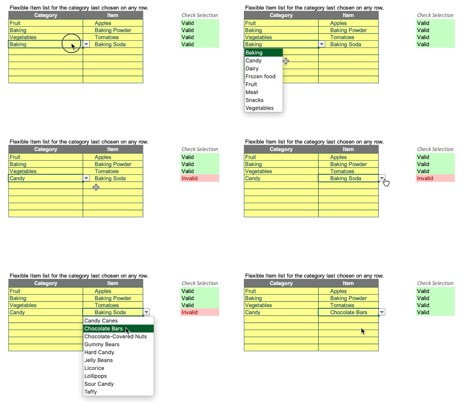
We add the following formula to check whether the value on each row is valid or not.
=SWITCH(ISBLANK(I14:I22)+ISBLANK(J14:J22),2,"",1,"Partial",0,IF(ISNA(XMATCH(I14:I22&J14:J22,tblFoods[Category]&tblFoods[Item],0)),"Invalid","Valid"))
The first part of the SWITCH function uses ISBLANK to check whether Category or Item or both are blank. If both are blank, the value will be 2, which will result with “” (blank). If only one is blank, the value will be 1, and the result of the formula will be “Partial”. If neither are blank, the value will be 0, and it will calculate the final part of the SWITCH:
IF(ISNA(XMATCH(I14:I22&J14:J22,tblFoods[Category]&tblFoods[Item],0)),"Invalid","Valid")).
XMATCH determines whether the combination of Category and Item can be found in the source data table. We use ISNA so that if XMATCH doesn’t find a match, it will result with “Invalid”. Otherwise it will result with “Valid”.
We added simple conditional formatting rules to add a little color if the result is Valid or Invalid.

Enter data in the correct sequence
Since we’re relying on the CELLfunction to determine the items in the drop-down, and the CELL function updates the result when Excel recalculates, our drop-down for Item will work great, but only when you enter data in the expected sequence. You need to pick a category first, and then an Item on the same row. For example, if you pick “Snacks” on the first row, but then pick an item on the 2ndrow, it will show snack items in the drop-down, even though you haven’t chosen a category on row 2.
Add a little VBA to make it more robust
This part is optional, but we can use VBA to make sure the drop-downs always show relevant items for the row where we’re entering data, even if we pick items out of order.
The VBA code below will cause Excel to recalculate whenever a cell with a drop-down is selected. This improves things because the formulae where we use the CELL function will be updated simply by selecting a cell with a drop-down. So, when we click on an Items cell, it doesn’t matter if the last cell we updated was the Category on the same row.
We won’t go explain the code in detail, but the important parts to know are:
- It will run when the selection changes on your sheet ('Worksheet_SelectionChange').
- If the cell has a DV drop-down list (ActiveCell.Validation.Type = xlValidateList), Excel will recalculate.
To add the code, follow these steps:
- Copy the code below
- Open the VBA editor. You can do this by pressing ALT+F11
- In the Project pane, find the worksheet where you’ve set up your drop-downs. Double-click the sheet, or right-click and choose 'View Code'
- In the code window, paste the code below.
Private Sub Worksheet_SelectionChange(ByVal Target As Range)
On Error GoTo ErrorHandler
If ActiveCell.Validation.Type = xlValidateList Then
Application.Calculate
End If
ErrorHandler:
'if there was an error just exit
Exit Sub
End Sub
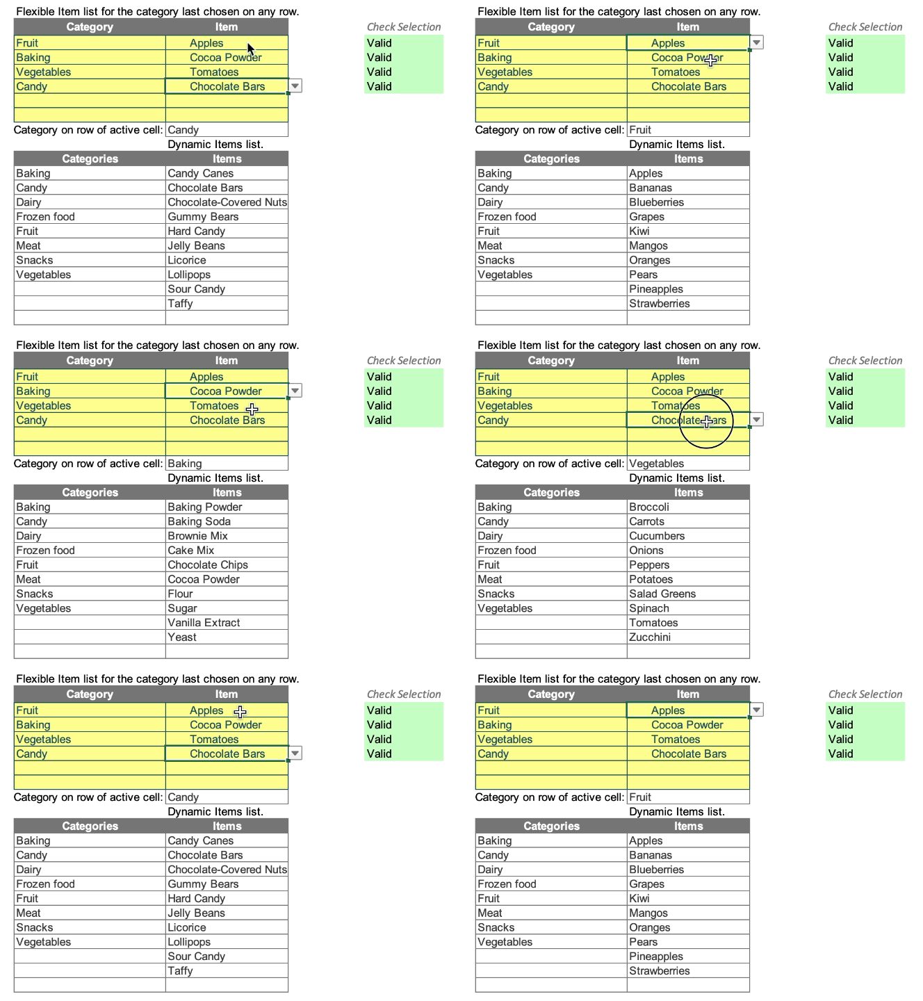
The gif below shows the effect of the VBA code. When the selection changes to a cell with a DV drop-down list, the cell below the table changes to the category on the row of the active cell. The list of Items below also changes, showing only items for that category. These are the items that would appear in the active cell’s drop-down list.
Our sample workbook contains more complex examples, where there are more than just 2 columns. In one example, we use different sheets for the cells that get the values for the lists and where we place the drop-downs. Have fun exploring the more complex examples.
We hope you enjoyed this article and find it useful. Thanks for reading. If you have questions or need help, please contact us at contact@sumproduct.com.

