
Weighted Averages Await
Sometimes, Excel problems are like buses. You don’t see a particular problem for a while and then suddenly, several come along, almost at the same time. That is exactly what happened with the subject of this article – calculating weighted averages where values change over time.
Our company often reviews / audits others’ financial models and over the past few weeks we have seen the same scenario on several occasions. Consider the following scenario:
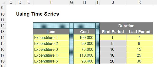
Here, various amounts of annual expenditure are incurred:
- $100,000 p.a. for the first seven years
- $90,000 p.a. for the next two years (years 8 and 9)
- $75,000 p.a. for the next six years (years 10 through 15)
- $110,000 p.a. for the next 10 years (years 16 to 25 inclusive)
- $98,400 p.a. for the final five years (years 26 to 30 inclusive).
The question is, what is the average annual expenditure? Several of our clients had simply used the AVERAGE function, but this takes the arithmetic average of the five values, i.e.
=AVERAGE(H14:H18)
which equates to $94,680. This is incorrect, as the five durations are not of similar length, and understates the true weighted average of $97,400 by nearly 3%, which may be significant in times of significant cash constraints, for example.
The correct average is easy enough to calculate with a helper column, viz.
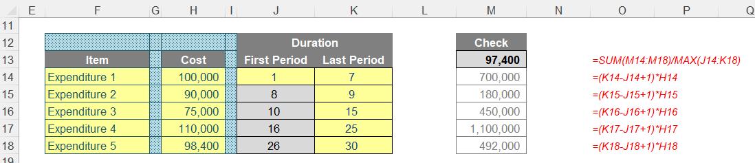
For each row, I may calculate the total costs by multiplying the cited expenditure by the duration (i.e. the number of relevant periods), e.g. for cell M14, the formula would be
=(K14-J14+1)*H14
At this point, do note that there is already an opportunity for a modelling error to occur. Many modellers will calculate the duration by subtracting the first period from the last period. This is not right, as this will exclude the first period: the number of periods is actually equal to the last period less the first period plus one, given by
K14-J14+1
in the above formula.
The value in cell M13 (above) simply adds these values together and divides by the total number of periods:
=SUM(M14:M18)/MAX(J14:K18)
That’s simple enough and probably not worthy of an article in its own right.
However, the reason that has driven me to write about this is that many do not use helper columns but try and write the entire calculation all in one cell. So, how do you do that?
I suggest the following formula:
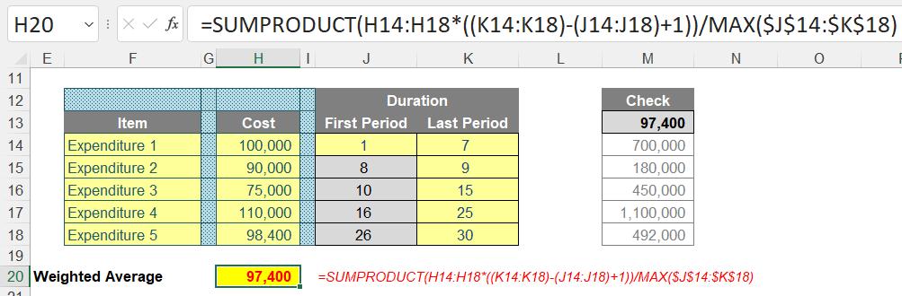
=SUMPRODUCT(H14:H18*((K14:K18)-(J14:J18)+1))/MAX($J$14:$K$18)
Just to explain, and as a reminder of SUMPRODUCT, consider the following side example:
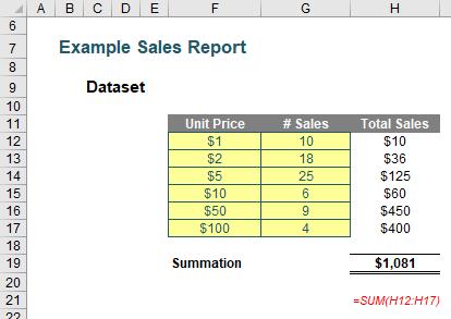
The sales in column H are simply the product of columns F and G, for example, the formula in cell H12 is simply =F12*G12. Then, to calculate the entire amount cell H19 sums column H. This could all be performed much quicker using the following formula:
=SUMPRODUCT(F12:F17,G12:G17)
You can multiply the vectors together instead:
=SUMPRODUCT(F12:F21*G12:G21)
This will produce the same result, and this is what is required in more complex scenarios.
Here, I have chosen to use the multiplication operator to make interpretation of the formula clearer, but using comma will achieve the same results. The formula
=SUMPRODUCT(H14:H18*((K14:K18)-(J14:J18)+1))/MAX($J$14:$K$18)
subtracts column J from column K and adds one to calculate the number of periods (i.e. the duration) on an array basis
=(K14:K18)-(J14:J18)+1
In our example,

this would produce the durations 7, 2, 6, 10 and 5 for rows 14, 15, 16, 17 and 18 respectively.
This duration is then multiplied by each cost on a row by row basis to obtain $700,000, $180,000, $450,000, $1,100,000 and $492,000 respectively for a grand total of $2,922,000:
=SUMPRODUCT(H14:H18*((K14:K18)-(J14:J18)+1))
Finally, this is divided by the total number of periods, which may be determined by calculating the maximum period number in the range (given by MAX($J$14:$K$18)),viz.
=SUMPRODUCT(H14:H18*((K14:K18)-(J14:J18)+1))/MAX($J$14:$K$18)
Please refer to the attached excel file for a modelled example.
Word to the Wise
This is a common calculation that is used to normalise amounts for valuation purposes, calculate depreciation, determine expected values, required funding, etc. Therefore, it is an essential technique to compute correctly.
However, many modellers make errors with this calculation as they strive to construct it all in one cell. To address this, I have created such a formula, but I would recommend it is preferable to step out such a calculation in a more longhand fashion (such as using helper column, detailed above) as it makes it both easier for end users to understand and lessens the risks of calculation errors.