What about US? Converting Dates to and from US Format
Dates can be awkward in Excel. Many countries use different formats from arguably the most prevalent: Day – Month – Year (DMY). One such country you might have heard of that differs from this “standard” is the United States, where it is more commonplace to use Month – Day – Year (MDY). Speaking from personal experience, I remember one project manager was nearly fired after he thought the deadline was 1 March 2015 when it was in fact 3 January 2015. This is the danger of 1/3/15, for example.
To show you how to overcome this problem, I will illustrate with converting US dates to what is often known as the “European” date format. Now I know many readers would prefer this to be the other way around. I apologize, but I am an Australian Brit with the appropriate regional settings on my machine and it’s a little awkward to perform screenshots that way. Don’t worry though – just follow me in reverse…
The problem becomes significant when you receive date data in a spreadsheet that is not recognized by your regional settings – or worse, it actually is, like my unfortunate project manager mentioned above. For me, my computer cannot make sense of US date formats such as
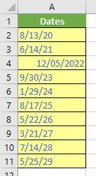
I have left the data in ‘General’ style deliberately so you can see only one entry, cell A4, is recognized as a number (date). The problem is, even that’s wrong as that represents 5 December 2022 not 12 May 2022.
How do I convert it? We could use Power Query / Get & Transform – but that’s not really what this series of articles is about. There is an easy way in Excel – but first, let’s start with a hard way…
In the screenshot below, I have managed to fix the issue:
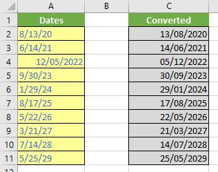
See? Easy. Oh sorry, I didn’t display the formula I used to do this in the image. Here it is for cell C2:
=VALUE(MID(IFERROR(TEXT(A2,"d/m/yy"),A2),FIND("@",SUBSTITUTE(IFERROR(TEXT(A2,"d/m/yy"),A2),"/","@",1))+1,FIND("/",SUBSTITUTE(IFERROR(TEXT(A2,"d/m/yy"),A2),"/","@",1))-FIND("@",SUBSTITUTE(IFERROR(TEXT(A2,"d/m/yy"),A2),"/","@",1))-1)&"/"&LEFT(IFERROR(TEXT(A2,"d/m/yy"),A2),FIND("@",SUBSTITUTE(IFERROR(TEXT(A2,"d/m/yy"),A2),"/","@",1))-1)&"/"&RIGHT(IFERROR(TEXT(A2,"d/m/yy"),A2),LEN(IFERROR(TEXT(A2,"d/m/yy"),A2))-FIND("/",SUBSTITUTE(IFERROR(TEXT(A2,"d/m/yy"),A2),"/","@",1))))
Any questions?
For those of you who have at this point decided that Excel is not for you, don’t stop reading here. I have provided the formula because I am fed up of the number of times I have read on the internet that this is not possible formulaically. Rubbish. You would just be a little insane to do it that way.
I have no intention of explaining this formula, suffice to say it only works for converting US dates to European dates, the text strings are delimited with “/” and do not contain “@” in the text string. If you want the conversion to go the other way, simply replace d/m/yy in all instances above with m/d/yy.
However, I think we are all agreed we need another – simpler! – way. Let’s start again. Back to the original data, I make a copy in cells C2:C11:
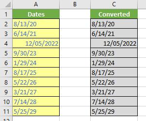
I do this so I may retain the original data (it’s always best to keep a copy in case you make a mistake).
Next, I highlight cells C1:C11 (including the header) and click on ‘Text to Columns’ in the ‘Data Tools’ grouping of the ‘Data’ tab of the Ribbon (Alt + A + E):

This generates the ‘Convert Text to Columns Wizard’ dialog box. In ‘Step 1’, choose the ‘Delimited’ option and click ‘Next’.
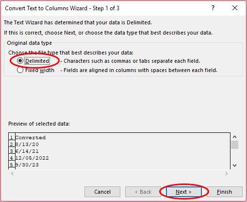
This means the data will be split into columns based upon a specified delimiter. Except we are going to cheat and not do that. In ‘Step 2’, uncheck all delimiters and then click ‘Next’:
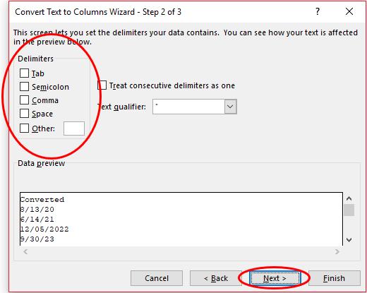
Now we come to the step that we actually want. We don’t use the ‘Text to Columns’ feature to split data into separate columns. No, I want Excel to recognize my data as dates.
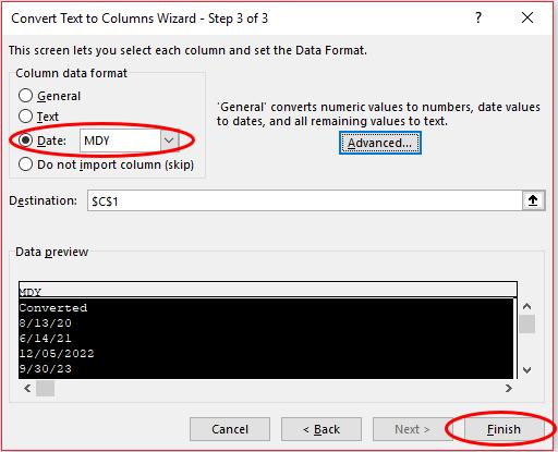
In this final step, select the ‘Date:’ option in the ‘Column data format’ and choose the date format that matches the data as it currently is – not what you want it to be. You are asking Excel to recognize it. In my case, the data is in Month – Day – Year format (MDY), so this is what I selected. Once you have chosen, click ‘Finish’:
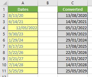
I think you will agree this far simpler than the formulaic approach, and more importantly, works for all date scenarios – as long as the original dates are formatted consistently.
As you keep working with dates, you will appreciate more and more the need for consistent dates, and the fact that they really aren’t that difficult to manipulate once you know the tricks.

