Multiple Multiple Criteria

This article revisits one of the most queried areas of modelling: how to sum data based upon multiple criteria. But this time around, it’s not quite as simple as that… By Liam Bastick, director with SumProduct Pty Ltd.

Query

I have looked through your previous article on working with Dealing with Multiple Criteria, but it doesn’t seem to answer my question. How can I sum amounts using a formula based upon multiple criteria for data situated in multiple rows within multiple worksheets?

Advice

This has been quite a popular topic and it is clear that the answer to this particular question isn’t that easy to come by. I will explain my solution using an illustration from the attached Excel file.

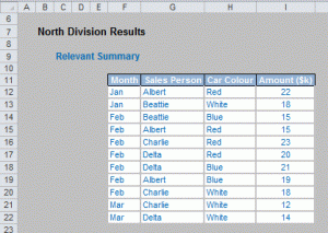
Let us imagine we run a car sales company with four divisions: North, South, East and West. Sales are reported in a similar fashion for each (North and South divisions are shown below):

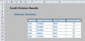
The month, associated sales person, car colour and cash amount of each sale is recorded. Note that the reports of each division may not be of equal length, but importantly the column headings of each table are in the same column of each spreadsheet (e.g. the month is always recorded in column F, the salesperson is always in column G, etc.). This is necessary for my solution to work.

Let’s build up the problem slowly.

Single Criterion, Single Data Source

I appreciate many readers will find this trivial, but for completeness I shall start here.

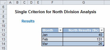
This is a simple use of the SUMIF function. For example, the formula in cell G12 in the illustration above is:

where North is the Excel worksheet containing North division’s sales data. For those unfamiliar with this useful function, SUMIF was discussed in Dealing with Multiple Criteria, the article mentioned previously (above). Alternative functions can be used but I am sticking with SUMIF as I will be using this and its sister function (SUMIFS) throughout this article. Essentially, all sales are added when the month of the sale matches the reporting month.

Multiple Criteria, Single Data Source

The next logical step is to increase the number of criteria (but still focus on just the one data source):

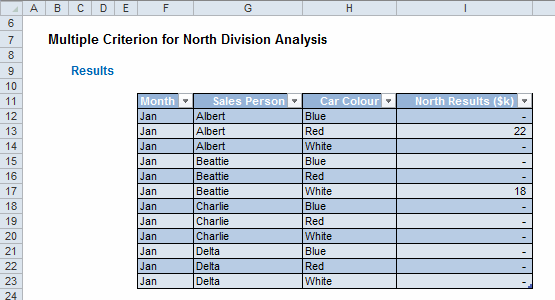
Again, there are many ways to solve this conundrum, but the one I have chosen has the following formula in cell I12:

Here, I have used the SUMIFS function (again, see Dealing with Multiple Criteria for more information), which deals with multiple criteria, here only summing data where the month, salesperson and car colour match the required criteria. Some may be amused to see I do not recommend our company’s namesake, SUMPRODUCT, here, but this function would not work on an entire column prior to its revision in Excel 2007.

Now, it gets more fun…

Single Criterion, Multiple Data Sources

Rather than make the jump to multiple criteria and multiple data sources all in one go, I thought it would be better to introduce one complication at a time:

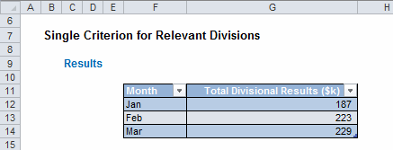
Before explaining the formula in G12 here, I would like to recommend an interim step. If I am to refer to multiple datasheets, I need to know the names of these worksheets. I suggest storing the worksheet names in a Table:

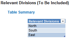
In the attached Excel file, this Table has been named Division_Table as this lists the divisions relevant for the analysis. It is intentional that I have not included all four divisions, but it is also important to note that the three divisions named (North, South and East here) must have identical names to the sheet tab names – otherwise, this solution will not work.

Tables represent a useful functionality, first introduced into Excel 2007 (for more information, see the previous article on Tables). Essentially, by listing data this way it allows users to add to the list (by putting, say, ‘West’ on the next line in my illustration) such that any referencing formulae will update the referenced list automatically.

Returning to this third example, namely multiple criteria based upon a single data source, the formula in cell G12 of my illustration is a little more sophisticated than the first two solutions:

You know you have created a monster when you nest three Excel functions inside a fourth. To work out what is going on, I will explain from the inside out (as this is how Excel will calculate this formula):

• INDIRECT (see Being Direct About INDIRECT) – This function produces an array of references such as ‘North’ column F, ‘South’ column F, etc. which can be used by the other functions. Note carefully that “‘” in the formula is inverted commas followed by an apostrophe (the syntax required in general for sheet names) followed by inverted commas.
• SUMIF – This function now applies the single criterion to the summation analysis. However, since it is not an array function, this will only report on one worksheet at a time (in my example, there are three sheets: ‘North’, ‘South’ and ‘East’).
• SUMPRODUCT – This function is necessary as this function is often referred to as a “pseudo array function” (arrays and array functions were discussed previously in Array of Light). What this means in practice here is that it will allow the SUMIF function to be performed across all three worksheets. SUMPRODUCT cannot be used without SUMIF however, as this function does not appear to work with multiple rows of data on multiple sheets (it only seems to consider the first cell of each selection on each sheet).
• IFERROR – This error trap ensures that if a worksheet listed in the Division_Table does not exist and / or there is a blank row, the formula will not produce a #REF! error for example.

Simple, n’est-ce pas..?

Multiple Criteria, Multiple Data Sources

So we now get to la pièce de résistance. If the reader has overcome the last hurdle this is a pièce de cake:

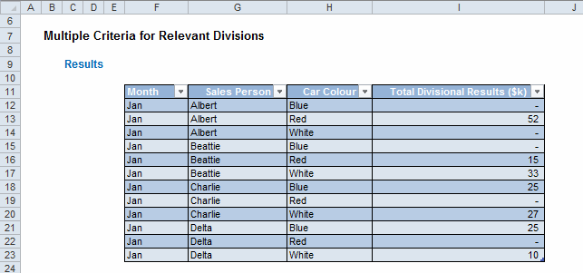
The formula in cell I12 here is just an extension of the last example:

Whilst the formula may look even more horrible upon first glance, essentially the SUMIFS function has merely replaced the SUMIF function, similar to the difference between the first two examples discussed above.

It’s not pretty, but it’s effective.

Word to the Wise

Given this solution uses Tables, IFERROR and the SUMIFS functions, this will only work in Excel 2007 and later versions of Excel.

Also, there are two other possible solutions to consider: PivotTables (see >Pivotal PivotTables) using data from multiple worksheets or creating a master data sheet as an interim step, where all data is recorded on one worksheet. I have produced this answer as this was faithful to the specific circumstances of the problem.

However, I would like to stress the age old rule: Keep It Simple Stupid (KISS). Having data on multiple worksheets complicates the problem and may not be a necessary complexity. Before writing opaque formulae such as the ones discussed above, always consider simplifying the model (structure) first.